Consolidation Breakout PRO — Clean Boxes + 200 EMA Trend Filter High-probability range breakout detector that draws perfect, always-visible consolidation boxes and only alerts when price breaks out with strong volume and (optionally) in the direction of the prevailing trend.
Features
Automatically draws and extends clean consolidation boxes in real time
Boxes stop extending the moment the breakout occurs — no more “ghost” lines
Optional but powerful 200 EMA trend filter (dramatically reduces false breakouts)
Stronger volume confirmation (default 1.8× the 20-period average, fully adjustable)
Auto-deletes old boxes so your chart stays perfectly clean even after hundreds of signals
Clear “BREAKOUT ↑” and “BREAKDOWN ↓” labels + ready-to-use alerts
Works on any market and any timeframe (best on 1H, 4H, Daily)
How to trade it (edge > 65 % when used correctly)
Wait for the labeled breakout candle to close
Enter on pullback/retest of the box edge (or on strong close + retest)
Stop-loss just outside the opposite side of the box
Take-profit: minimum 1:2, ideally measured move (box height added/subtracted) or trailing with the 20 EMA
This is the cleanest and most professional public consolidation breakout tool available in 2025 — no repainting, no lag, no chart clutter.
Created and continuously improved with love for the TradingView community.
Cari dalam skrip untuk "take profit"

Advanced Trading System - Volume Profile + BB + RSI + FVG + FibAdvanced Multi-Indicator Trading System with Volume Profile, Bollinger Bands, RSI, FVG & Fibonacci
Overview
This comprehensive trading indicator combines five powerful technical analysis tools into one unified system, designed to identify high-probability trading opportunities with precision entry and exit signals. The indicator integrates Volume Profile analysis, Bollinger Bands, RSI momentum, Fair Value Gaps (FVG), and Fibonacci retracement levels to provide traders with a complete market analysis framework.
Key Features
1. Volume Profile & Point of Control (POC)
Automatically calculates the Point of Control - the price level with the highest trading volume
Identifies Value Area High (VAH) and Value Area Low (VAL)
Updates dynamically based on customizable lookback periods
Helps identify key support and resistance zones where institutional traders are active
2. Bollinger Bands Integration
Standard 20-period Bollinger Bands with customizable multiplier
Identifies overbought and oversold conditions
Measures market volatility through band width
Signals generated when price approaches extreme levels
3. RSI Momentum Analysis
14-period Relative Strength Index with visual background coloring
Overbought (70) and oversold (30) threshold alerts
Integrated into buy/sell signal logic for confirmation
Real-time momentum tracking in info dashboard
4. Fair Value Gap (FVG) Detection
Automatically identifies bullish and bearish fair value gaps
Visual representation with colored boxes
Highlights imbalance zones where price may return
Used for high-probability entry confirmation
5. Fibonacci Retracement Levels
Auto-calculated based on recent swing high/low
Key levels: 23.6%, 38.2%, 50%, 61.8%, 78.6%
Perfect for identifying profit-taking zones
Dynamic lines that update with market movement
6. Smart Signal Generation
The indicator generates BUY and SELL signals based on multi-condition confluence:
BUY Signal Requirements:
Price near lower Bollinger Band
RSI in oversold territory (< 30)
High volume confirmation (optional)
Bullish FVG or POC alignment
SELL Signal Requirements:
Price near upper Bollinger Band
RSI in overbought territory (> 70)
High volume confirmation (optional)
Bearish FVG or POC alignment
7. Automated Take Profit Levels
Three dynamic profit targets: 1%, 2%, and 3%
Automatically calculated from entry price
Visual markers on chart
Individual alerts for each level
8. Comprehensive Alert System
The indicator includes 10+ alert types:
Buy signal alerts
Sell signal alerts
Take profit level alerts (TP1, TP2, TP3)
Fibonacci level cross alerts
RSI overbought/oversold alerts
Bullish/Bearish FVG detection alerts
9. Real-Time Info Dashboard
Live display of all key metrics
Color-coded for quick visual analysis
Shows RSI, BB Width, Volume ratio, POC, Fib levels
Current signal status (BUY/SELL/WAIT)
How to Use
Setup
Add the indicator to your chart
Adjust parameters based on your trading style and timeframe
Set up alerts by clicking "Create Alert" and selecting desired conditions
Recommended Timeframes
Scalping: 5m - 15m
Day Trading: 15m - 1H
Swing Trading: 4H - Daily
Parameter Customization
Volume Profile Settings:
Length: 100 (adjust for more/less historical data)
Rows: 24 (granularity of volume distribution)
Bollinger Bands:
Length: 20 (standard period)
Multiplier: 2.0 (adjust for tighter/wider bands)
RSI Settings:
Length: 14 (standard momentum period)
Overbought: 70
Oversold: 30
Fibonacci:
Lookback: 50 (swing high/low detection period)
Signal Settings:
Volume Filter: Enable/disable volume confirmation
Volume MA Length: 20 (for volume comparison)
Trading Strategy Examples
Strategy 1: Trend Reversal
Wait for BUY signal at lower Bollinger Band
Confirm with bullish FVG or POC support
Enter position
Take partial profits at Fib 38.2% and 50%
Exit remaining position at TP3 or SELL signal
Strategy 2: Breakout Confirmation
Monitor price approaching POC level
Wait for volume spike
Enter on signal confirmation with FVG alignment
Use Fibonacci levels for scaling out
Strategy 3: Range Trading
Identify POC as range midpoint
Buy at lower BB with oversold RSI
Sell at upper BB with overbought RSI
Use FVG zones for additional confirmation
Best Practices
✅ Do:
Use multiple timeframe analysis
Combine with price action analysis
Set stop losses below/above recent swing points
Scale out at Fibonacci levels
Wait for volume confirmation on signals
❌ Don't:
Trade every signal blindly
Ignore overall market context
Use on extremely low timeframes without testing
Neglect risk management
Trade during low liquidity periods
Risk Management
Always use stop losses
Risk no more than 1-2% per trade
Consider market conditions and volatility
Scale position sizes based on signal strength
Use the volume filter for additional confirmation
Technical Specifications
Pine Script Version: 6
Overlay: Yes (displays on main chart)
Max Boxes: 500 (for FVG visualization)
Max Lines: 500 (for Fibonacci levels)
Alerts: 10+ customizable conditions
Performance Notes
This indicator works best in:
Trending markets with clear momentum
High-volume trading sessions
Assets with good liquidity
When multiple signals align
Less effective in:
Extremely choppy/sideways markets
Low-volume periods
During major news events (high volatility)
Updates & Support
This indicator is actively maintained and updated. Future enhancements may include:
Additional volume profile features
More sophisticated FVG tracking
Enhanced alert customization
Backtesting integration
Disclaimer
This indicator is for educational and informational purposes only. It does not constitute financial advice. Past performance does not guarantee future results. Always conduct your own research and consider consulting with a financial advisor before making trading decisions. Trading involves substantial risk of loss.

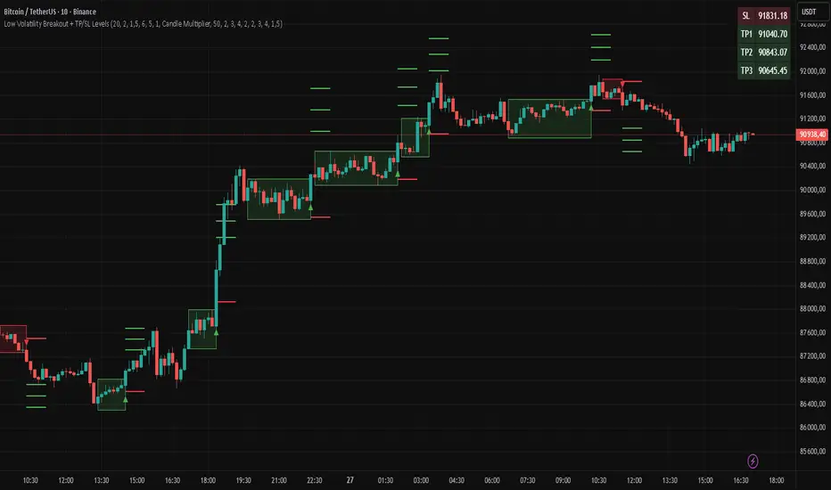
Low Volatility Breakout + TP/SL Levels█ OVERVIEW
"Low Volatility Breakout + TP/SL Levels" is a breakout indicator designed to detect and trade breakouts from periods of low volatility (consolidation). Unlike classic strategies based on fixed support/resistance levels, this indicator dynamically identifies consolidations characterized by small candle bodies and only generates a signal when the breakout occurs with a large, decisive candle. It also automatically plots 3 Take Profit levels and a Stop Loss (with two calculation modes), making it a complete breakout trading tool.
█ CONCEPTS
The strongest market moves most often start after a prolonged period of very low volatility — when candles become small and the market "falls asleep". The indicator first detects such consolidations (small bodies for at least X bars), draws a box around them, and then waits for a breakout with a candle significantly larger than the average. Additional filters (e.g., the box height cannot exceed the average candle body by too much) eliminate false consolidations and volatility traps. Immediately after the breakout, TP1, TP2, TP3, and SL levels are plotted.
█ FEATURES
Dynamic detection of low-volatility consolidations
- candles with small bodies (< average body × consolidationMultiplier)
- minimum number of bars in consolidation: confirmBars (default 5)
Automatic drawing of consolidation boxes
- green (bullish) or red (bearish) with transparent background (85)
- adjustable border thickness (border_width 1–5)
- box height filter (boxHeightMultiplier, default 6.0 × average body) – removes overly stretched/false consolidations
Breakout conditions
- current candle must be larger than average body × threshold (default 1.5)
- must be the largest candle in the entire consolidation
- must close above the highest high (long) or below the lowest low (short)
Breakout signals
- small green triangles below the bar (long)
- small red triangles above the bar (short)
Automatic Take Profit and Stop Loss levels (drawn 5 bars forward)
- two calculation modes:
• Candle Multiplier – based on average true range (high-low) over tp_sl_length period
• Percentage – fixed percentage from breakout close price (percentages must be manually adjusted to the asset and timeframe)
- 3 TP levels (default 2×, 3×, 4× or 2%, 3%, 4%)
- 1 SL level (default 2× or 1.5%)
Live TP/SL price table (top-right corner)
- displays exact current values of SL, TP1, TP2, TP3 immediately after each new signal
- colors identical to drawn lines (red background for SL, green for TP levels)
- updates automatically with every new breakout
Built-in alerts
- “Bullish Breakout Alert” and “Bearish Breakout Alert”
█ HOW TO USE
Add the indicator to your TradingView chart → Indicators → search “Low Volatility Breakout + TP/SL Levels”.
After each valid breakout you will immediately see:
- the colored box
- signal triangle
- horizontal TP/SL lines
- updated table in the top-right corner showing precise price levels for the current trade
Key settings to adjust:
Consolidation Settings
- Volatility Window (length) – period for average body calculation (default 20)
- Consolidation Multiplier – how small bodies must be to count as consolidation (default 2.0)
- Breakout Multiplier – minimum size of breakout candle (default 1.5)
- Box Height Multiplier – maximum allowed box height (default 6.0)
- Min Consolidation Bars – minimum bars required (default 5)
Risk Management Settings
- Choose TP/SL mode: Candle Multiplier or Percentage
- Adjust TP1–3 and SL multipliers/percentages to match your risk management style
Signal interpretation:
- Green triangle below bar + green box + green TP levels in table = long signal
- Red triangle above bar + red box + red SL level in table = short signal
- Boxes remain on chart until broken — they highlight accumulation/distribution zones
█ APPLICATIONS
- Trading breakouts from consolidation on all markets and timeframes
- Recommended to trade in the direction of the higher-timeframe trend or with additional confirmations (e.g., key level breaks). Aggressive mode (trading both directions) is also possible — provided box and TP/SL settings are properly optimized
- Experiment with different TP/SL ratios — higher reward-to-risk setups (e.g., SL 1×, TP3 6–8×) with lower win rate are often more profitable in the long run
- Strongly encourage testing various box parameters (consolidationMultiplier, boxHeightMultiplier, confirmBars) — small changes can dramatically affect signal frequency and quality
█ NOTES
Always test and optimize parameters for the specific instrument and timeframe.
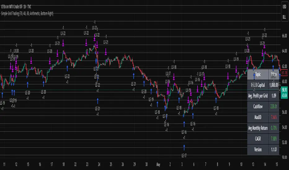
Simple Grid Trading v1.0 [PUCHON]Simple Grid Trading v1.0
Overview
This is a Long-Only Grid Trading Strategy developed in Pine Script v6 for TradingView. It is designed to profit from market volatility by placing a series of Buy Limit orders at predefined price levels. As the price drops, the strategy accumulates positions. As the price rises, it sells these positions at a profit.
Features
Grid Types : Supports both Arithmetic (equal price spacing) and Geometric (equal percentage spacing) grids.
Flexible Order Management : Uses strategy.order for precise control and prevents duplicate orders at the same level.
Performance Dashboard : A real-time table displaying key metrics like Capital, Cashflow, and Drawdown.
Advanced Metrics : Includes Max Drawdown (MaxDD) , Avg Monthly Return , and CAGR calculations.
Customizable : Fully adjustable price range, grid lines, and lot size.
Dashboard Metrics
The dashboard (default: Bottom Right) provides a quick snapshot of the strategy's performance:
Initial Capital : The starting capital defined in the strategy settings.
Lot Size : The fixed quantity of assets purchased per grid level.
Avg. Profit per Grid : The average realized profit for each closed trade.
Cashflow : The total realized net profit (closed trades only).
MaxDD : Maximum Drawdown . The largest percentage drop in equity (realized + unrealized) from a peak.
Avg Monthly Return : The average percentage return generated per month.
CAGR : Compound Annual Growth Rate . The mean annual growth rate of the investment over the specified time period.
Strategy Settings (Inputs)
Grid Settings
Upper Price : The highest price level for the grid.
Lower Price : The lowest price level for the grid.
Number of Grid Lines : The total number of levels (lines) in the grid.
Grid Type :
Arithmetic: Distance between lines is fixed in price terms (e.g., $10, $20, $30).
Geometric: Distance between lines is fixed in percentage terms (e.g., 1%, 2%, 3%).
Lot Size : The fixed amount of the asset to buy at each level.
Dashboard Settings
Show Dashboard : Toggle to hide/show the performance table.
Position : Choose where the dashboard appears on the chart (e.g., Bottom Right, Top Left).
How It Works
Initialization : On the first bar, the script calculates the price levels based on your Upper/Lower price and Grid Type.
Entry Logic :
The strategy places Buy Limit orders at every grid level below the current price.
It checks if a position already exists at a specific level to avoid "stacking" multiple orders on the same line.
Exit Logic :
For every Buy order, a corresponding Sell Limit (Take Profit) order is placed at the next higher grid level.
MaxDD Calculation :
The script continuously tracks the highest equity peak.
It calculates the drawdown on every bar (including intra-bar movements) to ensure accuracy.
Displayed as a percentage (e.g., 5.25%).
Disclaimer
This script is for educational and backtesting purposes only. Grid trading involves significant risk, especially in strong trending markets where the price may move outside your grid range. Always use proper risk management.
NIFTY Options Breakout StrategyThis strategy trades NIFTY 50 Options (CALL & PUT) using 5-minute breakout logic, strict trend filters, expiry-based symbol validation, and a dynamic trailing-profit engine.
1️⃣ Entry Logic
Only trades NIFTY 50 options, filtered automatically by symbol.
Trades only between 10:00 AM – 2:15 PM (5m bars).
Breakout trigger:
Price enters the buy breakout zone (high of last boxLookback bars ± buffer).
Trend filter:
Price must be above EMA50 or EMA200,
AND EMA50 ≥ EMA100 (to avoid weak conditions).
Optional strengthening:
EMA20>EMA50 OR EMA50>EMA100 recent cross can be enforced.
Higher-timeframe trend check:
EMA50 > EMA200 (bullish regime only).
Start trading options only after expiry–2 months (auto-parsed).
2️⃣ One Trade Per Day
Maximum 1 long trade per day.
No shorting (long-only strategy).
3️⃣ Risk Management — SL, TP & Trailing
Includes three types of exits:
🔹 A) Hard SL/TP
Hard Stop-Loss: -15%
Hard Take-Profit: +40%
🔹 B) Step-Ladder Trailing Profit
As the option price rises, trailing activates:
Max Profit Reached Exit Trigger When Falls To
≥ 35% ≤ 30%
≥ 30% ≤ 25%
≥ 25% ≤ 20%
≥ 20% ≤ 15%
≥ 15% ≤ 10%
≥ 5% ≤ 0%
🔹 C) Loss-Recovery Exit
If loss reaches –10% but then recovers to 0%, exit at breakeven.
4️⃣ Trend-Reversal Exit
If price closes below 5m EMA50, the long is exited instantly.
5️⃣ Optional Intraday Exit
EOD square-off at 3:15 PM.
6️⃣ Alerts for Automation
The strategy provides alerts for:
BUY entry
TP/SL/Trailing exit
EMA50 reversal exit
EOD exit

Market Energy & Direction DashboardMarket Energy & Direction Dashboard - Daytrading
Overview
A comprehensive real-time market internals dashboard that combines NYSE TICK, NYSE Advance-Decline (ADD) momentum, VIX direction, and relative volume into a single visual traffic light system with intelligent signal synthesis. Designed for active daytraders who need instant confirmation of market direction and energy based on momentum alignment across all major internals.
What It Does
This indicator synthesizes multiple market internals using directional momentum analysis rather than static thresholds to provide clear, actionable signals:
• Traffic Light System: Single glance confirmation of market state
o Bright Green: Maximum bullish - all internals aligned (TICK + ADD rising + VIX falling + volume)
o Bright Red: Maximum bearish - all internals aligned (TICK + ADD falling + VIX rising + volume)
o Yellow: Exhaustion warning - TICK at extremes, potential reversal imminent
o Moderate Colors: Partial alignment - some confirmation but not complete
o Gray: Choppy, neutral, or conflicting signals
• Real-Time Dashboard displays:
o Current TICK value with exhaustion warnings
o Current ADD with directional momentum indicator (↑ rising = breadth improving, ↓ falling = breadth deteriorating, ± compression)
o VIX level with directional indicator (↓ declining = bullish, ↑ rising = bearish, ± compression = neutral)
o Relative volume (current vs 20-period average)
o Composite status message synthesizing all data into clear directional summary
Key Features
✓ Momentum-based analysis - all indicators show direction/change, not just levels ✓ Intelligent signal hierarchy from "Maximum" to "Moderate" based on internal alignment ✓ ADD directional momentum - catches breadth shifts early, works in all market conditions ✓ VIX directional analysis - shows if fear is increasing, decreasing, or stagnant ✓ Color-coded traffic light for instant decision making ✓ Detects TICK/ADD divergences (conflicting signals = caution) ✓ Exhaustion warnings at extreme TICK levels (±1000+) ✓ Composite status messages - "Maximum Bull", "Strong Bull", "Moderate Bull", etc. ✓ Customizable thresholds for all parameters ✓ Moveable dashboard (9 position options) ✓ Built-in alerts for all signal strengths, exhaustion, and divergences
How To Use
Setup:
1. Add indicator to your main trading chart (SPY, ES, NQ, etc.)
2. Default settings work well for most traders, but you can customize:
o TICK Extreme Level (default 1000)
o ADD Compression Threshold (default 100 - detects when breadth is stagnant)
o VIX Elevated Level (default 20)
o VIX Compression Threshold (default 2% - detects low volatility)
o Volume Threshold (default 1.5x average)
3. Position dashboard wherever convenient on your chart
Reading The Signals:
Signal Hierarchy (Strongest to Weakest):
MAXIMUM SIGNALS ⭐ (Brightest colors - All 4 internals aligned)
• "✓ MAXIMUM BULL": TICK bullish + ADD rising (↑) + VIX falling (↓) + Volume elevated
o This is the holy grail setup - all momentum aligned, highest conviction longs
• "✓ MAXIMUM BEAR": TICK bearish + ADD falling (↓) + VIX rising (↑) + Volume elevated
o Perfect storm bearish - all momentum aligned, highest conviction shorts
STRONG SIGNALS (Bright colors - Core internals aligned)
• "✓ STRONG BULL": TICK bullish + ADD rising (↑)
o Strong confirmation even without VIX/volume - breadth supporting the move
• "✓ STRONG BEAR": TICK bearish + ADD falling (↓)
o Strong confirmation - both momentum and breadth deteriorating
MODERATE SIGNALS (Faded colors - Partial confirmation)
• "MODERATE BULL": TICK bullish but ADD not confirming direction
o Proceed with caution - momentum present but breadth questionable
• "MODERATE BEAR": TICK bearish but ADD not confirming direction
o Proceed with caution - selling but breadth not fully participating
WARNING SIGNALS
• "⚠ EXHAUSTION" (Yellow): TICK at ±1000+ extremes
o Potential reversal zone - prepare to fade or take profits
o Often marks blow-off tops or capitulation bottoms
NEUTRAL/AVOID
• "CHOPPY/NEUTRAL" (Gray): Conflicting signals or low conviction
o Stay out or reduce size significantly
Individual Indicator Interpretation:
TICK:
• Green: Bullish momentum (>+300)
• Red: Bearish momentum (<-300)
• Yellow: Exhaustion (±1000+)
• Gray: Neutral
ADD (Advance-Decline):
• Green (↑): Breadth improving - more stocks participating in the move
• Red (↓): Breadth deteriorating - fewer stocks participating
• Gray (±): Breadth stagnant - no clear participation trend
VIX:
• Green (↓): Fear declining - healthy environment for rallies
• Red (↑): Fear rising - risk-off mode, supports downward moves
• Gray (±): Volatility compression - often precedes explosive moves
Volume:
• Green: High conviction (>1.5x average)
• Gray: Low conviction
Trading Strategy:
1. Wait for "MAXIMUM" or "STRONG" signals for highest probability entries
o Maximum signals = go full size with confidence
o Strong signals = good conviction, normal position sizing
2. Confirm directional alignment:
o For longs: Want ADD ↑ (rising) and VIX ↓ (falling)
o For shorts: Want ADD ↓ (falling) and VIX ↑ (rising)
3. Use exhaustion warnings (yellow) to:
o Take profits on existing positions
o Prepare counter-trend entries
o Tighten stops
4. Avoid "MODERATE" signals unless you have strong conviction from other analysis
o These work best as confirmation for existing setups
o Not strong enough to initiate new positions alone
5. Never trade "CHOPPY/NEUTRAL" signals
o Gray means stay out - preserve capital
o Wait for clear alignment
6. Watch for divergences:
o Price making new highs but ADD ↓ (falling) = distribution warning
o Price making new lows but ADD ↑ (rising) = potential bottom
o Divergence alert will notify you
Best Practices:
• Use on 1-5 minute charts for daytrading
• Combine with your price action or technical setup (support/resistance, trendlines, patterns)
• The dashboard confirms when to take your setup, not what setup to take
• Most effective during regular market hours (9:30 AM - 4:00 PM ET) when volume is present
• The strongest edge comes from "MAXIMUM" signals - wait for these for best risk/reward
• Pay special attention to ADD direction - it's the most predictive breadth indicator
• VIX compression (gray ±) often signals upcoming volatility expansion - prepare for bigger moves
Customization Option
All thresholds are adjustable in settings:
• TICK Extreme: Higher = fewer exhaustion warnings (try 1200-1500 for less sensitivity)
• ADD Compression Threshold: Change detection sensitivity
o Default 100 = balanced
o Lower (50) = more sensitive to small breadth changes
o Higher (200-300) = only shows major breadth shifts
• VIX Elevated: Adjust for current volatility regime (15-25 typical range)
• VIX Compression Threshold:
o Default 2% = balanced
o Lower (0.5-1%) = catches subtle VIX changes
o Higher (3-5%) = only shows significant VIX moves
• Volume Threshold: Lower for quieter stocks/times, higher for more confirmation
Alerts Available
• Maximum Bullish: All 4 internals aligned bullish (TICK + ADD↑ + VIX↓ + Volume)
• Maximum Bearish: All 4 internals aligned bearish (TICK + ADD↓ + VIX↑ + Volume)
• Strong Bullish: TICK bullish + ADD rising
• Strong Bearish: TICK bearish + ADD falling
• Exhaustion Warning: TICK at extreme levels
• Divergence Warning: TICK and ADD directions conflicting
Understanding the Signal Synthesis
The indicator uses intelligent logic to combine all internals:
"MAXIMUM" Signals require:
• TICK direction (bullish/bearish)
• ADD momentum (rising/falling) in same direction
• VIX direction (falling for bulls, rising for bears)
• Volume elevated (>1.5x average)
"STRONG" Signals require:
• TICK direction (bullish/bearish)
• ADD momentum (rising/falling) in same direction
• (VIX and volume are bonuses but not required)
"MODERATE" Signals:
• TICK showing direction
• But ADD not confirming or contradicting
• Weakest actionable signal
This hierarchy ensures you know exactly how much conviction the market has behind any move.
Technical Details
• Pulls real-time data from NYSE TICK (USI:TICK), NYSE ADD (USI:ADD), and CBOE VIX
• ADD direction calculated using bar-to-bar change with compression detection
• VIX direction calculated using bar-to-bar percentage change
• Volume calculation uses 20-period simple moving average
• Dashboard updates every bar
• No repainting - all calculations based on closed bar data
Who This Is For
• Active daytraders of stocks, futures (ES/NQ), and options
• Scalpers needing quick directional confirmation with multiple internal alignment
• Swing traders looking to time intraday entries with maximum confluence
• Volatility traders who monitor VIX behavior
• Market makers and professionals who trade based on breadth and internals
• Anyone who monitors market internals but wants intelligent synthesis vs raw data
Tips For Success
Trading Philosophy:
• Quality over quantity - wait for "MAXIMUM" signals for best results
• One "MAXIMUM" signal trade is worth five "MODERATE" signal trades
• Gray/neutral is not a sign of missing opportunity - it's protecting your capital
Signal Confidence Levels:
1. MAXIMUM (95%+ confidence) - Trade these aggressively with full size
2. STRONG (80-85% confidence) - Trade these with normal position sizing
3. MODERATE (60-70% confidence) - Only if confirmed by strong technical setup
4. CHOPPY/NEUTRAL - Do not trade, wait for clarity
Advanced Techniques:
• Breadth divergences: Watch for price making new highs while ADD shows ↓ (falling) = major warning
• VIX/Price divergences: Rallies with rising VIX (↑) are usually false moves
• Volume confirmation: "MAXIMUM" signals with 2x+ volume are the absolute best
• Compression zones: When both ADD and VIX show compression (±), expect explosive breakout soon
• Sequential signals: Back-to-back "MAXIMUM" signals in same direction = strong trending day
Common Patterns:
• Opening surge with "MAXIMUM BULL" that shifts to "EXHAUSTION" (yellow) = fade the high
• Selloff with "MAXIMUM BEAR" followed by ADD ↑ (rising) divergence = potential reversal
• Choppy morning followed by "MAXIMUM" signal afternoon = best trending opportunity
Example Scenarios
Perfect Bull Entry:
• Bright green signal box
• TICK: +650
• ADD: +1200 (↑)
• VIX: 18.30 (↓)
• Volume: 2.3x
• Status: "✓ MAXIMUM BULL" → ALL SYSTEMS GO - Take aggressive long positions
Strong Bull (Good Confidence):
• Green signal box (slightly less bright)
• TICK: +500
• ADD: +800 (↑)
• VIX: 19.50 (±)
• Volume: 1.2x
• Status: "✓ STRONG BULL" → Good long setup - breadth confirming even without VIX/volume
Caution Bull (Moderate):
• Faded green signal box
• TICK: +400
• ADD: +900 (↓)
• VIX: 20.10 (↑)
• Volume: 0.9x
• Status: "MODERATE BULL" → CAUTION - TICK bullish but breadth deteriorating and VIX rising = weak rally
Exhaustion Warning:
• Yellow signal box
• TICK: +1350 ⚠
• ADD: +2100 (↑)
• VIX: 17.20 (↓)
• Volume: 1.8x
• Status: "⚠ EXHAUSTION" → Take profits or prepare to fade - TICK overextended despite good internals
Divergence Setup (Potential Reversal):
• Faded green signal
• TICK: +300
• ADD: +1800 (↓)
• VIX: 21.50 (↑)
• Volume: 1.6x
• Status: "MODERATE BULL" → WARNING - Price rallying but breadth collapsing and fear rising = distribution
Perfect Bear Entry:
• Bright red signal box
• TICK: -780
• ADD: -1600 (↓)
• VIX: 24.80 (↑)
• Volume: 2.5x
• Status: "✓ MAXIMUM BEAR" → Perfect short setup - all momentum bearish with conviction
Compression (Wait Mode):
• Gray signal box
• TICK: +50
• ADD: -200 (±)
• VIX: 16.40 (±)
• Volume: 0.7x
• Status: "CHOPPY/NEUTRAL" → STAY OUT - Volatility compression, no conviction, await breakout
Performance Optimization
Best Market Conditions:
• Works excellent in trending markets (up or down)
• Particularly powerful during high-volume sessions (first/last hours)
• "MAXIMUM" signals most reliable during 9:45-11:00 AM and 2:00-3:30 PM ET
Less Effective During:
• Lunch period (11:30 AM - 1:30 PM) - lower volume reduces signal quality
• Low-volatility environments - compression signals dominate
• Major news events in first 5 minutes - wait for internals to stabilize
Recommended Use Cases:
• Scalping: Trade only "MAXIMUM" signals for quick 5-15 minute moves
• Daytrading: Use "MAXIMUM" and "STRONG" signals for position entries
• Swing entries: Use "MAXIMUM" signals for optimal intraday entry timing
• Exit timing: Use "EXHAUSTION" (yellow) warnings to take profits
________________________________________
Pro Tip: Create a dedicated workspace with this indicator on SPY/ES/NQ charts. Set alerts for "MAXIMUM BULL", "MAXIMUM BEAR", and "EXHAUSTION" signals. Most professional traders only trade the "MAXIMUM" setups and ignore everything else - this alone can dramatically improve win rates.

DEMA ATR Strategy [PrimeAutomation]⯁ OVERVIEW
The DEMA ATR Strategy combines trend-following logic with adaptive volatility filters to identify strong momentum phases and manage trades dynamically.
It uses a Double Exponential Moving Average (DEMA) anchored to ATR volatility bands, creating a self-adjusting trend baseline.
When the adjusted DEMA shifts direction, the strategy enters positions and scales out profit in phases based on ATR-driven targets.
This system adapts to volatility, filters noise, and seeks sustained directional moves.
⯁ KEY FEATURES
DEMA-Volatility Hybrid Filter
Uses Double EMA with ATR expansion/compression logic to form a dynamic trend baseline.
Directional Shift Entries
Entries occur when the adjusted DEMA flips trend (bullish crossover or bearish crossunder vs its past value).
Noise Reduction Mechanism
ATR range caps extreme moves and prevents false flips during choppy volatility spikes.
Multi-Level Take Profits
Targets scale out positions at 1×, 2×, and 3× ATR multiples in the trade direction.
Volatility-Adaptive Targets
ATR multiplier ensures profit targets expand/contract based on market conditions.
Single-Direction Exposure
No pyramiding; the strategy flips position only when trend shifts.
Automated Trade Finalization
When all profit targets trigger, the position is fully closed.
⯁ STRATEGY LOGIC
Trend Direction:
DEMA baseline is modified using ATR upper/lower envelopes.
• If the adjusted DEMA rises above previous value → Bullish
• If it falls below previous value → Bearish
Entry Rules:
• Enter Long when bullish shift occurs and no long position exists
• Enter Short when bearish shift occurs and no short position exists
Take Profit Logic:
3 partial exits for each trade based on ATR:
• TP1 = ±1× ATR
• TP2 = ±2× ATR
• TP3 = ±3× ATR
Profit distribution: 30% / 30% / 40%
Exit Conditions:
• Exit when all TPs hit (full scale-out if sum of all TPs 100%)
• Opposite trend signal closes current trade and opens new one
⯁ WHEN TO USE
Trending environments
Medium–high volatility phases
Swing trading and intraday trend plays
Markets that respect momentum continuation (crypto, indices, FX majors)
⯁ CONCLUSION
This strategy blends DEMA trend recognition with ATR-based volatility adaptation to generate cleaner directional entries and structured take-profit exits. It is designed to capture momentum phases while avoiding noise-driven false signals, delivering a disciplined and scalable trend-following approach.

Crypto Grid 2025+ Long Only (Asym TP)Crypto Grid 2025+ Long Only (Asymmetric Take-Profit) is a long-only mean-reversion grid strategy designed for intraday cryptocurrency trading.
The core idea is to accumulate long positions as price moves downward within a locally defined price range and to exit positions on upward retracements.
The strategy automatically builds a multi-level grid between the highest and lowest price over a user-defined lookback period (“range length”). Each grid level acts as a potential entry point when price crosses it from above.
Key Features
1. Long-only grid logic
The strategy opens long positions only, progressively increasing exposure as price moves into lower grid levels.
2. Asymmetric take-profit mechanism
Instead of taking profit strictly at the next grid level, the strategy allows targeting multiple levels above the entry point. This increases the average profit per winning trade and shifts the reward-to-risk profile toward larger, less frequent wins.
3. Optional partial take-profit
A portion of each trade can be closed at the nearest grid level, while the remainder is held for a more distant asymmetric target. This balances consistency and profit potential.
4. Volume-based market filter
Entries can be restricted to periods of healthy market activity by requiring volume to exceed a moving-average baseline.
5. Capital-scaled position sizing
Position size is determined by risk percentage, grid spacing, and a dynamic sizing mode (original / conservative / aggressive).
6. Built-in risk controls
global stop below the lower boundary of the range,
global take-profit above the upper boundary,
automatic shutdown after a configurable loss-streak.
Market Philosophy
This strategy belongs to the mean-reversion family: it expects short-term overshoots to revert back toward mid-range liquidity zones.
It is not trend-following.
It performs best in choppy, range-bound, or slow-grinding markets — especially on liquid crypto pairs.
Recommended Use Cases
Short timeframes (1–15 minutes)
High-liquidity crypto pairs
Sideways or rotational price action
Exchanges with low fees (due to higher order count)
Not Intended For
Strong trending markets without pullbacks
Assets with thin order books
Use with leverage without additional risk controls
Summary
Crypto Grid 2025+ Long Only (Asymmetric TP) is a refined grid-based mean-reversion strategy optimized for modern crypto markets. Its asymmetric take-profit framework is specifically engineered to reduce the classical issue of “small wins and large occasional losses” found in traditional grid systems, giving it a more favorable long-term trade distribution.
PivotBoss VWAP Bands (Auto TF) - FixedWhat this indicator shows (high level)
The indicator plots a VWAP line and three bands above (R1, R2, R3) and three bands below (S1, S2, S3).
Band spacing is computed from STD(abs(VWAP − price), N) and multiplied by 1, 2 and 3 to form R1–R3 / S1–S3. The script is timeframe-aware: on 30m/1H charts it uses Weekly VWAP and weekly bands; on Daily charts it uses Monthly VWAP and monthly bands; otherwise it uses the session/chart VWAP.
VWAP = the market’s volume-weighted average price (a measure of fair value). Bands = volatility-scaled zones around that fair value.
Trading idea — concept summary
VWAP = fair value. Price above VWAP implies bullish bias; below VWAP implies bearish bias.
Bands = graded overbought/oversold zones. R1/S1 are near-term limits, R2/S2 are stronger, R3/S3 are extreme.
Use trend alignment + price action + volume to choose higher-probability trades. VWAP bands give location and magnitude; confirmations reduce false signals.
Entry rules (multiple strategies with examples)
A. Momentum breakout (trend-following) — preferred on trending markets
Setup: Price consolidates near or below R1 and then closes above R1 with above-average volume. Chart: 30m/1H (Weekly VWAP) or Daily (Monthly VWAP) depending on your timeframe.
Entry: Enter long at the close of the breakout bar that closes above R1.
Stop-loss: Place initial stop below the higher of (VWAP or recent swing low). Example: if price broke R1 at ₹1,200 and VWAP = ₹1,150, set stop at ₹1,145 (5 rupee buffer below VWAP) or below the last swing low if that is wider.
Target: Partial target at R2, full target at R3. Trail stop to VWAP or to R1 after price reaches R2.
Example numeric: Weekly VWAP = ₹1,150, R1 = ₹1,200, R2 = ₹1,260. Buy at ₹1,205 (close above R1), stop ₹1,145, target1 ₹1,260 (R2), target2 ₹1,320 (R3).
B. Mean-reversion fade near bands — for range-bound markets
Setup: Market is not trending (VWAP flatish). Price rallies up to R2 or R3 and shows rejection (pin bar, bearish engulfing) on increasing or neutral volume.
Entry: Enter short after a confirmed rejection candle that fails to sustain above R2 or R3 (prefer confirmation: close back below R1 or below the rejection candle low).
Stop-loss: Just above the recent high (e.g., 1–2 ATR or a fixed buffer above R2/R3).
Target: First target VWAP, second target S1. Reduce size if taking R3 fade as it’s an extreme.
Example numeric: VWAP = ₹950, R2 = ₹1,020. Price spikes to ₹1,025 and forms a bearish engulfing candle. Enter short at ₹1,015 after the next close below ₹1,020. Stop at ₹1,035, target VWAP ₹950.
C. Pullback entries in trending markets — higher probability
Setup: Price is above VWAP and trending higher (higher highs and higher lows). Price pulls back toward VWAP or S1 with decreasing downside volume and a reversal candle forms.
Entry: Long when price forms a bullish reversal (hammer/inside-bar) with a close back above the pullback candle.
Stop-loss: Below the pullback low (or below S2 if a larger stop is justified).
Target: VWAP then R1; if momentum resumes, trail toward R2/R3.
Example numeric: Price trending above Weekly VWAP at ₹1,400; pullback to S1 at ₹1,360. Enter long at ₹1,370 when a bullish candle closes; stop at ₹1,350; first target VWAP ₹1,400, second target R1 ₹1,450.
Exit rules and money management
Basic exit hierarchy
Hard stop exit — when price hits initial stop-loss. Always use.
Target exit — take partial profits at R1/R2 (for longs) or S1/S2 (for shorts). Use trailing stops for the remainder.
VWAP invalidation — if you entered long above VWAP and price returns and closes significantly below VWAP, consider exiting (condition depends on timeframe and trade size).
Price action exit — reversal patterns (strong opposite candle, bearish/bullish engulfing) near targets or beyond signals to exit.
Trailing rules
After price reaches R2, move stop to breakeven + a small buffer or to VWAP.
After price reaches R3, trail by 1 ATR or lock a defined profit percentage.
Position sizing & risk
Risk per trade: commonly 0.5–2% of account equity.
Determine position size by RiskAmount ÷ (EntryPrice − StopPrice).
If the stop distance is large (e.g., trading R3 fades), reduce position size.
Filters & confirmation (to reduce false signals)
Volume filter: For breakouts, require volume above short-term average (e.g., >20-period average). Breakouts on low volume are suspect.
Trend filter: Only take breakouts in the direction of the higher-timeframe trend (for example, use Daily/Weekly trend when trading 30m/1H).
Candle confirmation: Prefer entries on close of the confirming candle (not intrabar noise).
Multiple confirmations: When R1 break happens but RSI/plotted momentum indicator does not confirm, treat signal as lower probability.
Special considerations for timeframe-aware logic
On 30m/1H the script uses Weekly VWAP/bands. That means band levels change only on weekly candles — they are strong, structural levels. Treat R1/R2/R3 as significant and expect fewer, stronger signals.
On Daily, the script uses Monthly VWAP/bands. These are wider; trades should allow larger stops and smaller position sizes (or be used for swing trades).
On other intraday charts you get session VWAP (useful for intraday scalps).
Example: If you trade 1H and the Weekly R1 is at ₹2,400 while session VWAP is ₹2,350, a close above Weekly R1 represents a weekly-level breakout — prefer that for swing entries rather than scalps.
Example trade walkthrough (step-by-step)
Context: 1H chart, auto-mapped → Weekly VWAP used.
Weekly VWAP = ₹3,000; R1 = ₹3,080; R2 = ₹3,150.
Price consolidates below R1. A large bullish candle closes at ₹3,085 with volume 40% above the 20-bar average.
Entry: Buy at close ₹3,085.
Stop: Place stop at ₹2,995 (just under Weekly VWAP). Risk = ₹90.
Position size: If risking ₹900 per trade → size = 900 ÷ 90 = 10 units.
Targets: Partial take-profit at R2 = ₹3,150; rest trailed with stop moved to breakeven after R2 is hit.
If price reverses and closes below VWAP within two bars, exit immediately to limit drawdown.
When to avoid trading these signals
High-impact news (earnings, macro announcements) that can gap through bands unpredictably.
Thin markets with low volume — VWAP loses significance when volumes are extremely low.
When weekly/monthly bands are flat but intraday price is volatile without clear structure — prefer session VWAP on smaller timeframes.
Alerts & automation suggestions
Alert on close above R1 / below S1 (use the built-in alertcondition the script adds). For higher-confidence alerts, require volume filter in the alert condition.
Automated order rules (if you automate): use limit entry at breakout close plus a small slippage buffer, immediate stop order, and OCO for TP and SL.

EMA Trend Pro v1Here is a clear, professional English description you can copy-paste directly (suitable for sharing with friends, investors, brokers, or posting on TradingView):
EMA Trend Pro v5.0 – Strategy Overview
This is a trend-following strategy designed for 15-minute charts on assets like XAUUSD, NASDAQ, BTC, and ETH.
Entry Rules
Buy when the 7, 14, and 21-period EMAs are aligned upward and the 14-period EMA crosses above the 144-period EMA (with ADX > 20 and volume confirmation).
Sell short when the EMAs are aligned downward and the 14-period EMA crosses below the 144-period EMA.
Risk Management
Initial stop-loss is placed at 1.8 × ATR below (long) or above (short) the entry price.
Position size is calculated to risk a fixed percentage of equity per trade.
Profit-Taking & Trade Management
When price reaches 1:1 reward-to-risk, 30% of the position is closed.
At the same moment, the stop-loss for the remaining 70% is moved to the entry price (breakeven).
The remaining position is split:
50% targets 1:2 reward-to-risk
50% targets 1:3 reward-to-risk (allowing big wins during strong trends)
Visualization
Clean colored bars extend to the right showing entry, stop-loss, and three take-profit levels.
Price labels clearly display "Entry", "SL", "TP1 1:1", "TP2 1:2", and "TP3 1:3".
Only the current trade is displayed for a clean chart.
Key Advantages
High win rate due to breakeven protection after 1R
Excellent reward-to-risk ratio that lets winners run
Fully automated, works on any market with clear trends
Professional look, easy to understand and explain
Perfect for swing traders who want consistent profits with limited downside risk.
Feel free to use this description on TradingView, in your trading journal, or when explaining the strategy to others!
If you want a shorter version (e.g., for TradingView description box) or a Chinese version, just let me know — I’ll give it to you right away! 😊

EMA Trend Pro v5.0 5M ONLY — 策略版(1:1出30%+保本)Here is a clear, professional English description you can copy-paste directly (suitable for sharing with friends, investors, brokers, or posting on TradingView):
EMA Trend Pro v5.0 – Strategy Overview
This is a trend-following strategy designed for 15-minute charts on assets like XAUUSD, NASDAQ, BTC, and ETH.
Entry Rules
Buy when the 7, 14, and 21-period EMAs are aligned upward and the 14-period EMA crosses above the 144-period EMA (with ADX > 20 and volume confirmation).
Sell short when the EMAs are aligned downward and the 14-period EMA crosses below the 144-period EMA.
Risk Management
Initial stop-loss is placed at 1.8 × ATR below (long) or above (short) the entry price.
Position size is calculated to risk a fixed percentage of equity per trade.
Profit-Taking & Trade Management
When price reaches 1:1 reward-to-risk, 30% of the position is closed.
At the same moment, the stop-loss for the remaining 70% is moved to the entry price (breakeven).
The remaining position is split:
50% targets 1:2 reward-to-risk
50% targets 1:3 reward-to-risk (allowing big wins during strong trends)
Visualization
Clean colored bars extend to the right showing entry, stop-loss, and three take-profit levels.
Price labels clearly display "Entry", "SL", "TP1 1:1", "TP2 1:2", and "TP3 1:3".
Only the current trade is displayed for a clean chart.
Key Advantages
High win rate due to breakeven protection after 1R
Excellent reward-to-risk ratio that lets winners run
Fully automated, works on any market with clear trends
Professional look, easy to understand and explain
Perfect for swing traders who want consistent profits with limited downside risk.
Feel free to use this description on TradingView, in your trading journal, or when explaining the strategy to others!
If you want a shorter version (e.g., for TradingView description box) or a Chinese version, just let me know — I’ll give it to you right away! 😊

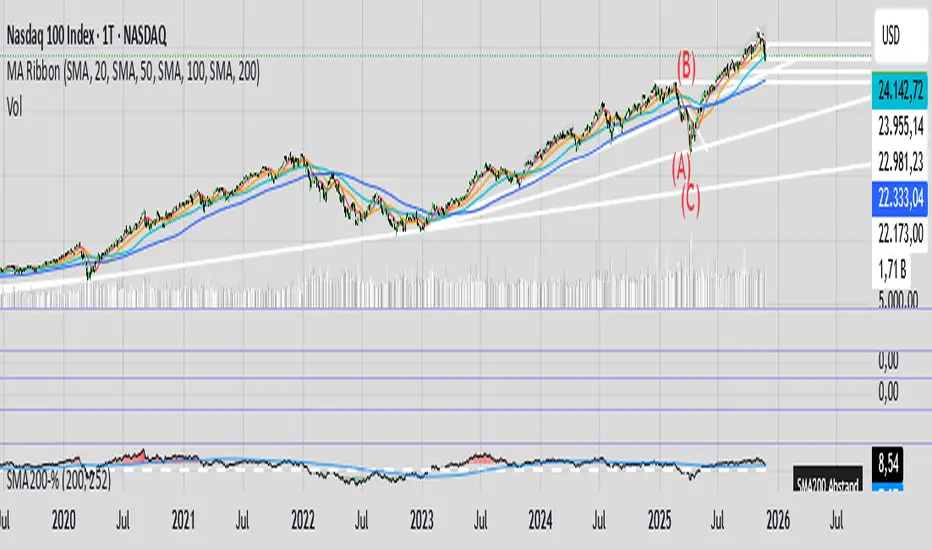
200SMA Distance OscillatorThe oscillator measures the percentage deviation of closing price x from SMA200.
The idea behind the oscillator was preceded by an analysis of how often MAs in the index hold/bounce or are broken through.
Basically, the idea was about index analysis, i.e., the macro picture of a market.
Who wants to buy individual stocks when the overall market is plummeting ;-)
Or in other words: How long are you long in a market? When is it time to take profits?
After the analysis of the stability of SMAs in the index was rather modest (ratio of just under 6:4 for bounce to breakout – overall in 20, 50, 100, and 200 frames from 2020 to 2025), it was noticeable that the percentage over- or underperformance was scalable, especially in indices.
And since indices generally move upwards, there were fixed limits for over- and underestimations – especially in the longer term (SMA200) – unlike with individual stocks.
It is therefore more a question of macro trends and less of short-term movements, e.g., in day trading.
It was now interesting to see at what percentage range counter-movements were likely – particularly in the positive range for profit-taking, but of course also in the negative range for entry into sold-off markets.
If, for example, closing prices around +25% above SMA200 were reached in the NDX, the probability is very high that the market has overreacted and an interim correction will follow – so the theory goes.
On the other hand, continuous levels of +5 to +10% are a product of healthy positive development in a bull market and do not necessarily require action.
The oscillator was specifically designed for the NDX, but can also be used for the SPX and others.
The style was based on the RSI, so that the color level rises from 10% to 20% (overbought/oversold principle).
Based on manually examined movements, the criteria were set as follows:
+/-10% = flow / no color background
> +/-10% = border areas / color background
The center line represents the 252 average of the percentage deviations and could also be used as a trigger, provided it has been historically examined and is valid.
The oscillator is very interesting because it behaves completely differently from one financial instrument to another and, as a result, also in the timeframes (4h, D, W).
It would probably make sense to change the flow and border levels in the code when using it outside of indices.
The fact is that the oscillator must be “adjusted” to each instrument in order to achieve its goal of providing the best possible prediction. “Adjusting” refers to the analysis of the levels at which an instrument/asset usually reacts.
As with all indicators and oscillators, it is advisable to take other indicators and, in particular, macro news into account when analyzing this development.
If I find any substantial correlations with other indicators, I will be happy to provide an update.
The idea came from me, the code from Grok.
The code is not 100% perfect, but the data (percentage deviation, color background) is correct according to initial analysis.
In the settings, you can make the lines of the plots invisible. This makes the oscillator clearer. You can also adjust the settings for the average line.
Mars Signals - Ultimate Institutional Suite v3.0(Joker)Comprehensive Trading Manual
Mars Signals – Ultimate Institutional Suite v3.0 (Joker)
## Chapter 1 – Philosophy & System Architecture
This script is not a simple “buy/sell” indicator.
Mars Signals – UIS v3.0 (Joker) is designed as an institutional-style analytical assistant that layers several methodologies into a single, coherent framework.
The system is built on four core pillars:
1. Smart Money Concepts (SMC)
- Detection of Order Blocks (professional demand/supply zones).
- Detection of Fair Value Gaps (FVGs) (price imbalances).
2. Smart DCA Strategy
- Combination of RSI and Bollinger Bands
- Identifies statistically discounted zones for scaling into spot positions or exiting shorts.
3. Volume Profile (Visible Range Simulation)
- Distribution of volume by price, not by time.
- Identification of POC (Point of Control) and high-/low-volume areas.
4. Wyckoff Helper – Spring
- Detection of bear traps, liquidity grabs, and sharp bullish reversals.
All four pillars feed into a Confluence Engine (Scoring System).
The final output is presented in the Dashboard, with a clear, human-readable signal:
- STRONG LONG 🚀
- WEAK LONG ↗
- NEUTRAL / WAIT
- WEAK SHORT ↘
- STRONG SHORT 🩸
This allows the trader to see *how many* and *which* layers of the system support a bullish or bearish bias at any given time.
## Chapter 2 – Settings Overview
### 2.1 General & Dashboard Group
- Show Dashboard Panel (`show_dash`)
Turns the dashboard table in the corner of the chart ON/OFF.
- Show Signal Recommendation (`show_rec`)
- If enabled, the textual signal (STRONG LONG, WEAK SHORT, etc.) is displayed.
- If disabled, you only see feature status (ON/OFF) and the current price.
- Dashboard Position (`dash_pos`)
Determines where the dashboard appears on the chart:
- `Top Right`
- `Bottom Right`
- `Top Left`
### 2.2 Smart Money (SMC) Group
- Enable SMC Strategy (`show_smc`)
Globally enables or disables the Order Block and FVG logic.
- Order Block Pivot Lookback (`ob_period`)
Main parameter for detecting key pivot highs/lows (swing points).
- Default value: 5
- Concept:
A bar is considered a pivot low if its low is lower than the lows of the previous 5 and the next 5 bars.
Similarly, a pivot high has a high higher than the previous 5 and the next 5 bars.
These pivots are used as anchors for Order Blocks.
- Increasing `ob_period`:
- Fewer levels.
- But levels tend to be more significant and reliable.
- In highly volatile markets (major news, war events, FOMC, etc.),
using values 7–10 is recommended to filter out weak levels.
- Show Fair Value Gaps (`show_fvg`)
Enables/disables the drawing of FVG zones (imbalances).
- Bullish OB Color (`c_ob_bull`)
- Color of Bullish Order Blocks (Demand Zones).
- Default: semi-transparent green (transparency ≈ 80).
- Bearish OB Color (`c_ob_bear`)
- Color of Bearish Order Blocks (Supply Zones).
- Default: semi-transparent red.
- Bullish FVG Color (`c_fvg_bull`)
- Color of Bullish FVG (upward imbalance), typically yellow.
- Bearish FVG Color (`c_fvg_bear`)
- Color of Bearish FVG (downward imbalance), typically purple.
### 2.3 Smart DCA Strategy Group
- Enable DCA Zones (`show_dca`)
Enables the Smart DCA logic and visual labels.
- RSI Length (`rsi_len`)
Lookback period for RSI (default: 14).
- Shorter → more sensitive, more noise.
- Longer → fewer signals, higher reliability.
- Bollinger Bands Length (`bb_len`)
Moving average period for Bollinger Bands (default: 20).
- BB Multiplier (`bb_mult`)
Standard deviation multiplier for Bollinger Bands (default: 2.0).
- For extremely volatile markets, values like 2.5–3.0 can be used so that only extreme deviations trigger a DCA signal.
### 2.4 Volume Profile (Visible Range Sim) Group
- Show Volume Profile (`show_vp`)
Enables the simulated Volume Profile bars on the right side of the chart.
- Volume Lookback Bars (`vp_lookback`)
Number of bars used to compute the Volume Profile (default: 150).
- Higher values → broader historical context, heavier computation.
- Row Count (`vp_rows`)
Number of vertical price segments (rows) to divide the total price range into (default: 30).
- Width (%) (`vp_width`)
Relative width of each volume bar as a percentage.
In the code, bar widths are scaled relative to the row with the maximum volume.
> Technical note: Volume Profile calculations are executed only on the last bar (`barstate.islast`) to keep the script performant even on higher timeframes.
### 2.5 Wyckoff Helper Group
- Show Wyckoff Events (`show_wyc`)
Enables detection and plotting of Wyckoff Spring events.
- Volume MA Length (`vol_ma_len`)
Length of the moving average on volume.
A bar is considered to have Ultra Volume if its volume is more than 2× the volume MA.
## Chapter 3 – Smart Money Strategy (Order Blocks & FVG)
### 3.1 What Is an Order Block?
An Order Block (OB) represents the footprint of large institutional orders:
- Bullish Order Block (Demand Zone)
The last selling region (bearish candle/cluster) before a strong upward move.
- Bearish Order Block (Supply Zone)
The last buying region (bullish candle/cluster) before a strong downward move.
Institutions and large players place heavy orders in these regions. Typical price behavior:
- Price moves away from the zone.
- Later returns to the same zone to fill unfilled orders.
- Then continues the larger trend.
In the script:
- If `pl` (pivot low) forms → a Bullish OB is created.
- If `ph` (pivot high) forms → a Bearish OB is created.
The box is drawn:
- From `bar_index ` to `bar_index`.
- Between `low ` and `high `.
- `extend=extend.right` extends the OB into the future, so it acts as a dynamic support/resistance zone.
- Only the last 4 OB boxes are kept to avoid clutter.
### 3.2 Order Block Color Guide
- Semi-transparent Green (`c_ob_bull`)
- Represents a Bullish Order Block (Demand Zone).
- Interpretation: a price region with a high probability of bullish reaction.
- Semi-transparent Red (`c_ob_bear`)
- Represents a Bearish Order Block (Supply Zone).
- Interpretation: a price region with a high probability of bearish reaction.
Overlap (Multiple OBs in the Same Area)
When two or more Order Blocks overlap:
- The shared area appears visually denser/stronger.
- This suggests higher order density.
- Such zones can be treated as high-priority levels for entries, exits, and stop-loss placement.
### 3.3 Demand/Supply Logic in the Scoring Engine
is_in_demand = low <= ta.lowest(low, 20)
is_in_supply = high >= ta.highest(high, 20)
- If current price is near the lowest lows of the last 20 bars, it is considered in a Demand Zone → positive impact on score.
- If current price is near the highest highs of the last 20 bars, it is considered in a Supply Zone → negative impact on score.
This logic complements Order Blocks and helps the Dashboard distinguish whether:
- Market is currently in a statistically cheap (long-friendly) area, or
- In a statistically expensive (short-friendly) area.
### 3.4 Fair Value Gaps (FVG)
#### Concept
When the market moves aggressively:
- Some price levels are skipped and never traded.
- A gap between wicks/shadows of consecutive candles appears.
- These regions are called Fair Value Gaps (FVGs) or Imbalances.
The market generally “dislikes” imbalance and often:
- Returns to these zones in the future.
- Fills the gap (rebalance).
- Then resumes its dominant direction.
#### Implementation in the Code
Bullish FVG (Yellow)
fvg_bull_cond = show_smc and show_fvg and low > high and close > high
if fvg_bull_cond
box.new(bar_index , high , bar_index, low, ...)
Core condition:
`low > high ` → the current low is above the high of two bars ago; the space between them is an untraded gap.
Bearish FVG (Purple)
fvg_bear_cond = show_smc and show_fvg and high < low and close < low
if fvg_bear_cond
box.new(bar_index , low , bar_index, high, ...)
Core condition:
`high < low ` → the current high is below the low of two bars ago; again a price gap exists.
#### FVG Color Guide
- Transparent Yellow (`c_fvg_bull`) – Bullish FVG
Often acts like a magnet for price:
- Price tends to retrace into this zone,
- Fill the imbalance,
- And then continue higher.
- Transparent Purple (`c_fvg_bear`) – Bearish FVG
Price tends to:
- Retrace upward into the purple area,
- Fill the imbalance,
- And then resume downward movement.
#### Trading with FVGs
- FVGs are *not* standalone entry signals.
They are best used as:
- Targets (take-profit zones), or
- Reaction areas where you expect a pause or reversal.
Examples:
- If you are long, a bearish FVG above is often an excellent take-profit zone.
- If you are short, a bullish FVG below is often a good cover/exit zone.
### 3.5 Core SMC Trading Templates
#### Reversal Long
1. Price trades down into a green Order Block (Demand Zone).
2. A bullish confirmation candle (Close > Open) forms inside or just above the OB.
3. If this zone is close to or aligned with a bullish FVG (yellow), the signal is reinforced.
4. Entry:
- At the close of the confirmation candle, or
- Using a limit order near the upper boundary of the OB.
5. Stop-loss:
- Slightly below the OB.
- If the OB is broken decisively and price consolidates below it, the zone loses validity.
6. Targets:
- The next FVG,
- Or the next red Order Block (Supply Zone) above.
#### Reversal Short
The mirror scenario:
- Price rallies into a red Order Block (Supply).
- A bearish confirmation candle forms (Close < Open).
- FVG/premium structure above can act as a confluence.
- Stop-loss goes above the OB.
- Targets: lower FVGs or subsequent green OBs below.
## Chapter 4 – Smart DCA Strategy (RSI + Bollinger Bands)
### 4.1 Smart DCA Concept
- Classic DCA = buying at fixed time intervals regardless of price.
- Smart DCA = scaling in only when:
- Price is statistically cheaper than usual, and
- The market is in a clear oversold condition.
Code logic:
rsi_val = ta.rsi(close, rsi_len)
= ta.bb(close, bb_len, bb_mult)
dca_buy = show_dca and rsi_val < 30 and close < bb_lower
dca_sell = show_dca and rsi_val > 70 and close > bb_upper
Conditions:
- DCA Buy – Smart Scale-In Zone
- RSI < 30 → oversold.
- Close < lower Bollinger Band → price has broken below its typical volatility envelope.
- DCA Sell – Overbought/Distribution Zone
- RSI > 70 → overbought.
- Close > upper Bollinger Band → price is extended far above the mean.
### 4.2 Visual Representation on the Chart
- Green “DCA” Label Below Candle
- Shape: `labelup`.
- Color: lime background, white text.
- Meaning: statistically attractive level for laddered spot entries or short exits.
- Red “SELL” Label Above Candle
- Warning that the market is in an extended, overbought condition.
- Suitable for profit-taking on longs or considering short entries (with proper confluence and risk management).
- Light Green Background (`bgcolor`)
- When `dca_buy` is true, the candle background turns very light green (high transparency).
- This helps visually identify DCA Zones across the chart at a glance.
### 4.3 Practical Use in Trading
#### Spot Trading
Used to build a better average entry price:
- Every time a DCA label appears, allocate a fixed portion of capital (e.g., 2–5%).
- Combining DCA signals with:
- Green OBs (Demand Zones), and/or
- The Volume Profile POC
makes the zone structurally more important.
#### Futures Trading
- Longs
- Use DCA Buy signals as low-risk zones for opening or adding to longs when:
- Price is inside a green OB, or
- The Dashboard already leans LONG.
- Shorts
- Use DCA Sell signals as:
- Exit zones for longs, or
- Areas to initiate shorts with stops above structural highs.
## Chapter 5 – Volume Profile (Visible Range Simulation)
### 5.1 Concept
Traditional volume (histogram under the chart) shows volume over time.
Volume Profile shows volume by price level:
- At which prices has the highest trading activity occurred?
- Where did buyers and sellers agree the most (High Volume Nodes – HVNs)?
- Where did price move quickly due to low participation (Low Volume Nodes – LVNs)?
### 5.2 Implementation in the Script
Executed only when `show_vp` is enabled and on the last bar:
1. The last `vp_lookback` bars (default 150) are processed.
2. The minimum low and maximum high over this window define the price range.
3. This price range is divided into `vp_rows` segments (e.g., 30 rows).
4. For each row:
- All bars are scanned.
- If the mid-price `(high + low ) / 2` falls inside a row, that bar’s volume is added to the row total.
5. The row with the greatest volume is stored as `max_vol_idx` (the POC row).
6. For each row, a volume box is drawn on the right side of the chart.
### 5.3 Color Scheme
- Semi-transparent Orange
- The row with the maximum volume – the Point of Control (POC).
- Represents the strongest support/resistance level from a volume perspective.
- Semi-transparent Blue
- Other volume rows.
- The taller the bar → the higher the volume → the stronger the interest at that price band.
### 5.4 Trading Applications
- If price is above POC and retraces back into it:
→ POC often acts as support, suitable for long setups.
- If price is below POC and rallies into it:
→ POC often acts as resistance, suitable for short setups or profit-taking.
HVNs (Tall Blue Bars)
- Represent areas of equilibrium where the market has spent time and traded heavily.
- Price tends to consolidate here before choosing a direction.
LVNs (Short or Nearly Empty Bars)
- Represent low participation zones.
- Price often moves quickly through these areas – useful for targeting fast moves.
## Chapter 6 – Wyckoff Helper – Spring
### 6.1 Spring Concept
In the Wyckoff framework:
- A Spring is a false break of support.
- The market briefly trades below a well-defined support level, triggers stop losses,
then sharply reverses upward as institutional buyers absorb liquidity.
This movement:
- Clears out weak hands (retail sellers).
- Provides large players with liquidity to enter long positions.
- Often initiates a new uptrend.
### 6.2 Code Logic
Conditions for a Spring:
1. The current low is lower than the lowest low of the previous 50 bars
→ apparent break of a long-standing support.
2. The bar closes bullish (Close > Open)
→ the breakdown was rejected.
3. Volume is significantly elevated:
→ `volume > 2 × volume_MA` (Ultra Volume).
When all conditions are met and `show_wyc` is enabled:
- A pink diamond is plotted below the bar,
- With the label “Spring” – one of the strongest long signals in this system.
### 6.3 Trading Use
- After a valid Spring, markets frequently enter a meaningful bullish phase.
- The highest quality setups occur when:
- The Spring forms inside a green Order Block, and
- Near or on the Volume Profile POC.
Entries:
- At the close of the Spring bar, or
- On the first pullback into the mid-range of the Spring candle.
Stop-loss:
- Slightly below the Spring’s lowest point (wick low plus a small buffer).
## Chapter 7 – Confluence Engine & Dashboard
### 7.1 Scoring Logic
For each bar, the script:
1. Resets `score` to 0.
2. Adjusts the score based on different signals.
SMC Contribution
if show_smc
if is_in_demand
score += 1
if is_in_supply
score -= 1
- Being in Demand → `+1`
- Being in Supply → `-1`
DCA Contribution
if show_dca
if dca_buy
score += 2
if dca_sell
score -= 2
- DCA Buy → `+2` (strong, statistically driven long signal)
- DCA Sell → `-2`
Wyckoff Spring Contribution
if show_wyc
if wyc_spring
score += 2
- Spring → `+2` (entry of strong money)
### 7.2 Mapping Score to Dashboard Signal
- score ≥ 2 → STRONG LONG 🚀
Multiple bullish conditions aligned.
- score = 1 → WEAK LONG ↗
Some bullish bias, but only one layer clearly positive.
- score = 0 → NEUTRAL / WAIT
Rough balance between buying and selling forces; staying flat is usually preferable.
- score = -1 → WEAK SHORT ↘
Mild bearish bias, suited for cautious or short-term plays.
- score ≤ -2 → STRONG SHORT 🩸
Convergence of several bearish signals.
### 7.3 Dashboard Structure
The dashboard is a two-column table:
- Row 0
- Column 0: `"Mars Signals"` – black background, white text.
- Column 1: `"UIS v3.0"` – black background, yellow text.
- Row 1
- Column 0: `"Price:"` (light grey background).
- Column 1: current closing price (`close`) with a semi-transparent blue background.
- Row 2
- Column 0: `"SMC:"`
- Column 1:
- `"ON"` (green) if `show_smc = true`
- `"OFF"` (grey) otherwise.
- Row 3
- Column 0: `"DCA:"`
- Column 1:
- `"ON"` (green) if `show_dca = true`
- `"OFF"` (grey) otherwise.
- Row 4
- Column 0: `"Signal:"`
- Column 1: signal text (`status_txt`) with background color `status_col`
(green, red, teal, maroon, etc.)
- If `show_rec = false`, these cells are cleared.
## Chapter 8 – Visual Legend (Colors, Shapes & Actions)
For quick reading inside TradingView, the visual elements are described line by line instead of a table.
Chart Element: Green Box
Color / Shape: Transparent green rectangle
Core Meaning: Bullish Order Block (Demand Zone)
Suggested Trader Response: Look for longs, Smart DCA adds, closing or reducing shorts.
Chart Element: Red Box
Color / Shape: Transparent red rectangle
Core Meaning: Bearish Order Block (Supply Zone)
Suggested Trader Response: Look for shorts, or take profit on existing longs.
Chart Element: Yellow Area
Color / Shape: Transparent yellow zone
Core Meaning: Bullish FVG / upside imbalance
Suggested Trader Response: Short take-profit zone or expected rebalance area.
Chart Element: Purple Area
Color / Shape: Transparent purple zone
Core Meaning: Bearish FVG / downside imbalance
Suggested Trader Response: Long take-profit zone or temporary supply region.
Chart Element: Green "DCA" Label
Color / Shape: Green label with white text, plotted below the candle
Core Meaning: Smart ladder-in buy zone, DCA buy opportunity
Suggested Trader Response: Spot DCA entry, partial short exit.
Chart Element: Red "SELL" Label
Color / Shape: Red label with white text, plotted above the candle
Core Meaning: Overbought / distribution zone
Suggested Trader Response: Take profit on longs, consider initiating shorts.
Chart Element: Light Green Background (bgcolor)
Color / Shape: Very transparent light-green background behind bars
Core Meaning: Active DCA Buy zone
Suggested Trader Response: Treat as a discount zone on the chart.
Chart Element: Orange Bar on Right
Color / Shape: Transparent orange horizontal bar in the volume profile
Core Meaning: POC – price with highest traded volume
Suggested Trader Response: Strong support or resistance; key reference level.
Chart Element: Blue Bars on Right
Color / Shape: Transparent blue horizontal bars in the volume profile
Core Meaning: Other volume levels, showing high-volume and low-volume nodes
Suggested Trader Response: Use to identify balance zones (HVN) and fast-move corridors (LVN).
Chart Element: Pink "Spring" Diamond
Color / Shape: Pink diamond with white text below the candle
Core Meaning: Wyckoff Spring – liquidity grab and potential major bullish reversal
Suggested Trader Response: One of the strongest long signals in the suite; look for high-quality long setups with tight risk.
Chart Element: STRONG LONG in Dashboard
Color / Shape: Green background, white text in the Signal row
Core Meaning: Multiple bullish layers in confluence
Suggested Trader Response: Consider initiating or increasing longs with strict risk management.
Chart Element: STRONG SHORT in Dashboard
Color / Shape: Red background, white text in the Signal row
Core Meaning: Multiple bearish layers in confluence
Suggested Trader Response: Consider initiating or increasing shorts with a logical, well-placed stop.
## Chapter 9 – Timeframe-Based Trading Playbook
### 9.1 Timeframe Selection
- Scalping
- Timeframes: 1M, 5M, 15M
- Objective: fast intraday moves (minutes to a few hours).
- Recommendation: focus on SMC + Wyckoff.
Smart DCA on very low timeframes may introduce excessive noise.
- Day Trading
- Timeframes: 15M, 1H, 4H
- Provides a good balance between signal quality and frequency.
- Recommendation: use the full stack – SMC + DCA + Volume Profile + Wyckoff + Dashboard.
- Swing Trading & Position Investing
- Timeframes: Daily, Weekly
- Emphasis on Smart DCA + Volume Profile.
- SMC and Wyckoff are used mainly to fine-tune swing entries within larger trends.
### 9.2 Scenario A – Scalping Long
Example: 5-Minute Chart
1. Price is declining into a green OB (Bullish Demand).
2. A candle with a long lower wick and bullish close (Pin Bar / Rejection) forms inside the OB.
3. A Spring diamond appears below the same candle → very strong confluence.
4. The Dashboard shows at least WEAK LONG ↗, ideally STRONG LONG 🚀.
5. Entry:
- On the close of the confirmation candle, or
- On the first pullback into the mid-range of that candle.
6. Stop-loss:
- Slightly below the OB.
7. Targets:
- Nearby bearish FVG above, and/or
- The next red OB.
### 9.3 Scenario B – Day-Trading Short
Recommended Timeframes: 1H or 4H
1. The market completes a strong impulsive move upward.
2. Price enters a red Order Block (Supply).
3. In the same zone, a purple FVG appears or remains unfilled.
4. On a lower timeframe (e.g., 15M), RSI enters overbought territory and a DCA Sell signal appears.
5. The main timeframe Dashboard (1H) shows WEAK SHORT ↘ or STRONG SHORT 🩸.
Trade Plan
- Open a short near the upper boundary of the red OB.
- Place the stop above the OB or above the last swing high.
- Targets:
- A yellow FVG lower on the chart, and/or
- The next green OB (Demand) below.
### 9.4 Scenario C – Swing / Investment with Smart DCA
Timeframes: Daily / Weekly
1. On the daily or weekly chart, each time a green “DCA” label appears:
- Allocate a fixed fraction of your capital (e.g., 3–5%) to that asset.
2. Check whether this DCA zone aligns with the orange POC of the Volume Profile:
- If yes → the quality of the entry zone is significantly higher.
3. If the DCA signal sits inside a daily green OB, the probability of a medium-term bottom increases.
4. Always build the position laddered, never all-in at a single price.
Exits for investors:
- Near weekly red OBs or large purple FVG zones.
- Ideally via partial profit-taking rather than closing 100% at once.
### 9.5 Case Study 1 – BTCUSDT (15-Minute)
- Context: Price has sold off down towards 65,000 USD.
- A green OB had previously formed at that level.
- Near the lower boundary of this OB, a partially filled yellow FVG is present.
- As price returns to this region, a Spring appears.
- The Dashboard shifts from NEUTRAL / WAIT to WEAK LONG ↗.
Plan
- Enter a long near the OB low.
- Place stop below the Spring low.
- First target: a purple FVG around 66,200.
- Second (optional) target: the first red OB above that level.
### 9.6 Case Study 2 – Meme Coin (PEPE – 4H)
- After a strong pump, price enters a corrective phase.
- On the 4H chart, RSI drops below 30; price breaks below the lower Bollinger Band → a DCA label prints.
- The Volume Profile shows the POC at approximately the same level.
- The Dashboard displays STRONG LONG 🚀.
Plan
- Execute laddered buys in the combined DCA + POC zone.
- Place a protective stop below the last significant swing low.
- Target: an expected 20–30% upside move towards the next red OB or purple FVG.
## Chapter 10 – Risk Management, Psychology & Advanced Tuning
### 10.1 Risk Management
No signal, regardless of its strength, replaces risk control.
Recommendations:
- In futures, do not expose more than 1–3% of account equity to risk per trade.
- Adjust leverage to the volatility of the instrument (lower leverage for highly volatile altcoins).
- Place stop-losses in zones where the idea is clearly invalidated:
- Below/above the relevant Order Block or Spring, not randomly in the middle of the structure.
### 10.2 Market-Specific Parameter Tuning
- Calmer Markets (e.g., major FX pairs)
- `ob_period`: 3–5.
- `bb_mult`: 2.0 is usually sufficient.
- Highly Volatile Markets (Crypto, news-driven assets)
- `ob_period`: 7–10 to highlight only the most robust OBs.
- `bb_mult`: 2.5–3.0 so that only extreme deviations trigger DCA.
- `vol_ma_len`: increase (e.g., to ~30) so that Spring triggers only on truly exceptional
volume spikes.
### 10.3 Trading Psychology
- STRONG LONG 🚀 does not mean “risk-free”.
It means the probability of a successful long, given the model’s logic, is higher than average.
- Treat Mars Signals as a confirmation and context system, not a full replacement for your own decision-making.
- Example of disciplined thinking:
- The Dashboard prints STRONG LONG,
- But price is simultaneously testing a multi-month macro resistance or a major negative news event is imminent,
- In such cases, trade smaller, widen stops appropriately, or skip the trade.
## Chapter 11 – Technical Notes & FAQ
### 11.1 Does the Script Repaint?
- Order Blocks and Springs are based on completed pivot structures and confirmed candles.
- Until a pivot is confirmed, an OB does not exist; after confirmation, behavior is stable under classic SMC assumptions.
- The script is designed to be structurally consistent rather than repainting signals arbitrarily.
### 11.2 Computational Load of Volume Profile
- On the last bar, the script processes up to `vp_lookback` bars × `vp_rows` rows.
- On very low timeframes with heavy zooming, this can become demanding.
- If you experience performance issues:
- Reduce `vp_lookback` or `vp_rows`, or
- Temporarily disable Volume Profile (`show_vp = false`).
### 11.3 Multi-Timeframe Behavior
- This version of the script is not internally multi-timeframe.
All logic (OB, DCA, Spring, Volume Profile) is computed on the active timeframe only.
- Practical workflow:
- Analyze overall structure and key zones on higher timeframes (4H / Daily).
- Use lower timeframes (15M / 1H) with the same tool for timing entries and exits.
## Conclusion
Mars Signals – Ultimate Institutional Suite v3.0 (Joker) is a multi-layer trading framework that unifies:
- Price structure (Order Blocks & FVG),
- Statistical behavior (Smart DCA via RSI + Bollinger),
- Volume distribution by price (Volume Profile with POC, HVN, LVN),
- Liquidity events (Wyckoff Spring),
into a single, coherent system driven by a transparent Confluence Scoring Engine.
The final output is presented in clear, actionable language:
> STRONG LONG / WEAK LONG / NEUTRAL / WEAK SHORT / STRONG SHORT
The system is designed to support professional decision-making, not to replace it.
Used together with strict risk management and disciplined execution,
Mars Signals – UIS v3.0 (Joker) can serve as a central reference manual and operational guide
for your trading workflow, from scalping to swing and investment positioning.
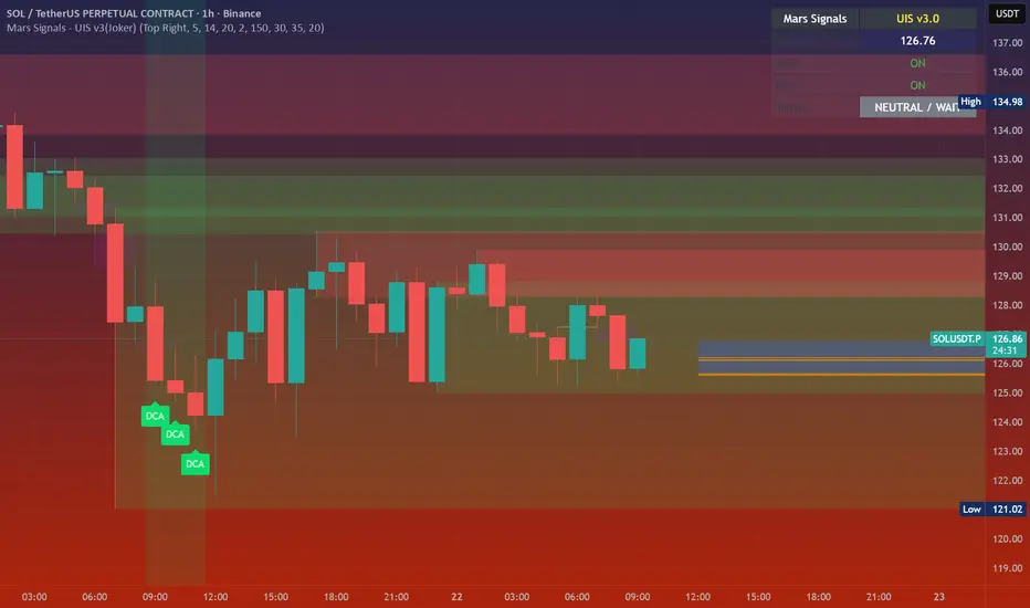
Sani Momentum Target System [wjdtks255]Sani Momentum Target System Explanation & Trading Method
The Sani Momentum Target System is a momentum-based trading indicator that helps traders identify trend changes and determine precise entry points, stop-loss levels, and multiple profit targets.
Key Features:
Smoothed Price Calculation: Utilizes a glide-like smoothing function to reduce noise in price data.
Moving Averages: Calculates fast and slow EMAs on the smoothed price; the difference creates an oscillator.
Signal Line: A simple moving average smooths the oscillator to generate a signal line.
Trend Signals:
Buy signal when oscillator crosses above the signal line.
Sell signal when oscillator crosses below the signal line.
Entry, Stop Loss, Target Levels:
Entry price is set at current close on signal.
Stop loss is set by multiplying ATR by 2 against trend direction.
Three take profit targets (T1, T2, T3) are set by user-defined multiples of ATR.
Visual Display: Includes colored horizontal lines and labels for entry, stop loss, and targets.
Bars are colored by trend direction, and triangular markers show buy/sell signals.
How To Use This Indicator:
Entry: Place trades in the direction of the signal (long on buy, short on sell).
Stop Loss: Use the ATR-based stop loss line to minimize downside risk.
Profit Taking: Scale out profits or exit trades at target levels T1, T2, and T3.
Trend Confirmation: Confirm with oscillator trend direction before entry to avoid false signals.
Parameter Adjustment: Modify smoothing lengths, ATR period, and target multipliers to fit your trading style and timeframe.
Final Notes:
This indicator streamlines momentum trading by providing clear price targets and risk levels visually.
Always backtest strategies and apply proper risk management.
Suitable across asset classes: stocks, forex, cryptocurrencies.
If you want detailed guidance or customization, feel free to ask!

ATR (No Gap) - Advanced Volatility IndicatorA customizable Average True Range indicator that eliminates gap distortion between trading sessions, providing cleaner volatility measurements for intraday and swing traders.
Key Features:
Gap Filtering: Optional toggle to ignore overnight/weekend gaps that distort volatility readings
EMA Smoothing: Defaults to EMA for more responsive volatility tracking (also supports RMA and SMA)
Half ATR Display: Shows 50% ATR value for quick stop-loss and take-profit calculations
Clean Value Table: Real-time values displayed on chart with configurable decimal precision
Flexible Settings: Customize length, smoothing method, and display options
Ideal for:
Setting dynamic stop losses and take profits
Position sizing based on current volatility
Comparing gap vs. no-gap volatility measurements
Trading instruments with large overnight gaps (indices, forex, crypto)
Use this indicator to get a more accurate picture of intraday volatility without the noise from session gaps!

Range Trading StrategyOVERVIEW
The Range Trading Strategy is a systematic trading approach that identifies price ranges
from higher timeframe candles or trading sessions, tracks pivot points, and generates
trading signals when range extremes are mitigated and confirmed by pivot levels.
CORE CONCEPT
The strategy is based on the principle that when a candle (or session) closes within the
range of the previous candle (or session), that previous candle becomes a "range" with
identifiable high and low extremes. When price breaks through these extremes, it creates
trading opportunities that are confirmed by pivot levels.
RANGE DETECTION MODES
1. HTF (Higher Timeframe) Mode:
Automatically selects a higher timeframe based on the current chart timeframe
Uses request.security() to fetch HTF candle data
Range is created when an HTF candle closes within the previous HTF candle's range
The previous HTF candle's high and low become the range extremes
2. Sessions Mode:
- Divides the trading day into 4 sessions (UTC):
* Session 1: 00:00 - 06:00 (6 hours)
* Session 2: 06:00 - 12:00 (6 hours)
* Session 3: 12:00 - 20:00 (8 hours)
* Session 4: 20:00 - 00:00 (4 hours, spans midnight)
- Tracks high, low, and close for each session
- Range is created when a session closes within the previous session's range
- The previous session's high and low become the range extremes
PIVOT DETECTION
Pivots are detected based on candle color changes (bullish/bearish transitions):
1. Pivot Low:
Created when a bullish candle appears after a bearish candle
Pivot low = minimum of the current candle's low and previous candle's low
The pivot bar is the actual bar where the low was formed (current or previous bar)
2. Pivot High:
Created when a bearish candle appears after a bullish candle
Pivot high = maximum of the current candle's high and previous candle's high
The pivot bar is the actual bar where the high was formed (current or previous bar)
IMPORTANT: There is always only ONE active pivot high and ONE active pivot low at any
given time. When a new pivot is created, it replaces the previous one.
RANGE CREATION
A range is created when:
(HTF Mode) An HTF candle closes within the previous HTF candle's range AND a new HTF
candle has just started
(Sessions Mode) A session closes within the previous session's range AND a new session
has just started
Or Range Can Be Created when the Extreme of Another Range Gets Mitigated and We Have a Pivot low Just Above the Range Low or Pivot High just Below the Range High
Range Properties:
rangeHigh: The high extreme of the range
rangeLow: The low extreme of the range
highStartTime: The timestamp when the range high was actually formed (found by looping
backwards through bars)
lowStartTime: The timestamp when the range low was actually formed (found by looping
backwards through bars)
highMitigated / lowMitigated: Flags tracking whether each extreme has been broken
isSpecial: Flag indicating if this is a "special range" (see Special Ranges section)
RANGE MITIGATION
A range extreme is considered "mitigated" when price interacts with it:
High is mitigated when: high >= rangeHigh (any interaction at or above the level)
Low is mitigated when: low <= rangeLow (any interaction at or below the level)
Mitigation can happen:
At the moment of range creation (if price is already beyond the extreme)
At any point after range creation when price touches the extreme
SIGNAL GENERATION
1. Pending Signals:
When a range extreme is mitigated, a pending signal is created:
a) BEARISH Pending Signal:
- Triggered when: rangeHigh is mitigated
- Confirmation Level: Current pivotLow
- Signal is confirmed when: close < pivotLow
- Stop Loss: Current pivotHigh (at time of confirmation)
- Entry: Short position
Signal Confirmation
b) BULLISH Pending Signal:
- Triggered when: rangeLow is mitigated
- Confirmation Level: Current pivotHigh
- Signal is confirmed when: close > pivotHigh
- Stop Loss: Current pivotLow (at time of confirmation)
- Entry: Long position
IMPORTANT: There is only ever ONE pending bearish signal and ONE pending bullish signal
at any given time. When a new pending signal is created, it replaces the previous one
of the same type.
2. Signal Confirmation:
- Bearish: Confirmed when price closes below the pivot low (confirmation level)
- Bullish: Confirmed when price closes above the pivot high (confirmation level)
- Upon confirmation, a trade is entered immediately
- The confirmation line is drawn from the pivot bar to the confirmation bar
TRADE EXECUTION
When a signal is confirmed:
1. Position Management:
- Any existing position in the opposite direction is closed first
- Then the new position is entered
2. Stop Loss:
- Bearish (Short): Stop at pivotHigh
- Bullish (Long): Stop at pivotLow
3. Take Profit:
- Calculated using Risk:Reward Ratio (default 2:1)
- Risk = Distance from entry to stop loss
- Target = Entry ± (Risk × R:R Ratio)
- Can be disabled with "Stop Loss Only" toggle
4. Trade Comments:
- "Range Bear" for short trades
- "Range Bull" for long trades
SPECIAL RANGES
Special ranges are created when:
- A range high is mitigated AND the current pivotHigh is below the range high
- A range low is mitigated AND the current pivotLow is above the range low
In these cases:
- The pivot value is stored in an array (storedPivotHighs or storedPivotLows)
- A "special range" is created with only ONE extreme:
* If pivotHigh < rangeHigh: Creates a range with rangeHigh = pivotLow, rangeLow = na
* If pivotLow > rangeLow: Creates a range with rangeLow = pivotHigh, rangeHigh = na
- Special ranges can generate signals just like normal ranges
- If a special range is mitigated on the creation bar or the next bar, it is removed
entirely without generating signals (prevents false signals)
Special Ranges
REVERSE ON STOP LOSS
When enabled, if a stop loss is hit, the strategy automatically opens a trade in the
opposite direction:
1. Long Stop Loss Hit:
- Detects when: position_size > 0 AND position_size <= 0 AND low <= longStopLoss
- Action: Opens a SHORT position
- Stop Loss: Current pivotHigh
- Trade Comment: "Reverse on Stop"
2. Short Stop Loss Hit:
- Detects when: position_size < 0 AND position_size >= 0 AND high >= shortStopLoss
- Action: Opens a LONG position
- Stop Loss: Current pivotLow
- Trade Comment: "Reverse on Stop"
The reverse trade uses the same R:R ratio and respects the "Stop Loss Only" setting.
VISUAL ELEMENTS
1. Range Lines:
- Drawn from the time when the extreme was formed to the mitigation point (or current
time if not mitigated)
- High lines: Blue (or mitigated color if mitigated)
- Low lines: Red (or mitigated color if mitigated)
- Style: SOLID
- Width: 1
2. Confirmation Lines:
- Drawn when a signal is confirmed
- Extends from the pivot bar to the confirmation bar
- Bearish: Red, solid line
- Bullish: Green, solid line
- Width: 1
- Can be toggled on/off
STRATEGY SETTINGS
1. Range Detection Mode:
- HTF: Uses higher timeframe candles
- Sessions: Uses trading session boundaries
2. Auto HTF:
- Automatically selects HTF based on current chart timeframe
- Can be disabled to use manual HTF selection
3. Risk:Reward Ratio:
- Default: 2.0 (2:1)
- Minimum: 0.5
- Step: 0.5
4. Stop Loss Only:
- When enabled: Trades only have stop loss (no take profit)
- Trades close on stop loss or when opposite signal confirms
5. Reverse on Stop Loss:
- When enabled: Hitting a stop loss opens opposite trade with stop at opposing pivot
6. Max Ranges to Display:
- Limits the number of ranges kept in memory
- Oldest ranges are purged when limit is exceeded
KEY FEATURES
1. Dynamic Pivot Tracking:
- Pivots update on every candle color change
- Always maintains one high and one low pivot
2. Range Lifecycle:
- Ranges are created when price closes within previous range
- Ranges are tracked until mitigated
- Mitigation creates pending signals
- Signals are confirmed by pivot levels
3. Signal Priority:
- Only one pending signal of each type at a time
- New signals replace old ones
- Confirmation happens on close of bar
4. Position Management:
- Closes opposite positions before entering new trades
- Tracks stop loss levels for reverse functionality
- Respects pyramiding = 1 (only one position per direction)
5. Time-Based Drawing:
- Uses time coordinates instead of bar indices for line drawing
- Prevents "too far from current bar" errors
- Lines can extend to any historical point
USAGE NOTES
- Best suited for trending and ranging markets
- Works on any timeframe, but HTF mode adapts automatically
- Sessions mode is ideal for intraday trading
- Pivot detection requires clear candle color changes
- Range detection requires price to close within previous range
- Signals are generated on bar close, not intra-bar
The strategy combines range identification, pivot tracking, and signal confirmation to
create a systematic approach to trading breakouts and reversals based on price structure, past performance does not in any way predict future performance

MACD Volume VWAP Scalping (2min) by Obiii📘 Strategy Description (for TradingView)
MACD Volume VWAP Scalping Strategy (2-Minute Intraday Momentum)
This strategy is designed for scalpers and short-term intraday traders who focus on capturing small, high-probability moves during the most active hours of the trading session — typically between 9:45 AM and 11:30 AM (New York time).
The system combines three key momentum confirmations:
MACD crossovers to detect short-term trend shifts,
Volume spikes to validate real market participation, and
VWAP / EMA alignment to filter trades in the direction of the prevailing intraday trend.
🔹 Entry Logic
Long Entry:
MACD line crosses above the signal line
Both MACD and Signal are above zero
Current volume > average of the last 10 candles
Price is above VWAP and (optionally) above EMA 9 and EMA 20
Short Entry:
MACD line crosses below the signal line
Both MACD and Signal are below zero
Current volume > average of the last 10 candles
Price is below VWAP and (optionally) below EMA 9 and EMA 20
🎯 Exit Logic
Fixed Take Profit: +0.25%
Fixed Stop Loss: -0.15% to -0.20%
Optionally, switch to the 5-minute chart after entry to monitor momentum and manage exits more smoothly.
⚙️ Recommended Settings
Timeframe: 2 minutes (entries), 5 minutes (monitoring)
Market Session: 9:45 AM – 11:30 AM EST
Assets: Highly liquid instruments such as SPY, QQQ, NVDA, TSLA, AAPL, or large-cap momentum stocks.
💡 Notes
This is a momentum-based scalping strategy — precision and discipline are key.
It performs best in high-volume environments where clear direction emerges after the morning volatility settles.
The system can be fine-tuned for different profit targets, MACD settings, or volume thresholds depending on volatility.

Pearson SL/TP📘 Description
Pearson SL/TP — Advanced Correlation-Based Strategy with Full Risk Management
The Pearson SL/TP indicator is an advanced market analysis tool that combines Pearson correlation, volatility-based stop/target levels, and dynamic signal strength evaluation.
It is designed for traders who want to visualize potential momentum shifts and risk/reward zones in a single, integrated chart.
🔍 Core Concept
This script measures the **Pearson correlation coefficient between recent price movements and time progression, highlighting potential trend exhaustion or momentum reversals when the correlation reaches extreme values.
* High positive correlation (near +1) → price moving steadily upward → possible overbought condition.
* High negative correlation (near -1) → price moving steadily downward → possible oversold condition.
When these extremes are reached, and confirmed by several internal filters, the script generates LONG or SHORT signals with fully calculated Stop Loss and Take Profit levels.
⚙️ Main Features
📈 Signal Generation
* Uses Pearson correlation as a primary indicator of trend intensity.
* Detects potential reversal zones when correlation crosses user-defined thresholds.
* Optional divergence confirmation enhances signal reliability.
💰 Risk Management
* Stop Loss (SL) and Take Profits (TP1 & TP2) automatically adapt to volatility using the ATR (Average True Range).
* Dynamic risk/reward ratios help assess trade quality.
* Adjustable multipliers let you fine-tune your risk parameters.
🧠 Signal Strength Analysis
Each signal is graded from Weak to Very Strong based on four factors:
1. Volume activity
2. Trend alignment
3. Pearson momentum
4. Correlation change intensity
🎨 Visualization
* Overbought / Oversold background zones
* Signal arrows (LONG / SHORT)
* SL / TP** price levels and labels
* Interactive dashboard** displaying:
* Current Pearson value
* Market state (Overbought / Oversold / Neutral)
* Signal strength
* Latest trade data (Entry, SL, TP1, TP2, Risk:Reward)
🔔 Alerts
Built-in alerts for:
* Confirmed LONG / SHORT signals
* Bullish / Bearish divergences
🧩 Customization
All major parameters — including **Pearson length, thresholds, ATR multipliers, and visual options — are fully customizable.
This allows you to adapt the indicator to any market, timeframe, or trading style.

Victoria RSI Hybrid Pro – Momentum + Volume + DivergenceConditions and Actions:
RSI > 50 → Bullish regime → Consider Calls
RSI < 50 → Bearish regime → Consider Puts
RSI crosses up → Momentum shift up → Buy confirmation
RSI crosses down → Momentum shift down → Sell confirmation
RSI > 70 → Overbought → Take profits
RSI < 30 → Oversold → Watch for reversal
Bullish divergence → Hidden upward momentum → Reversal watch
Bearish divergence → Hidden downward momentum → Reversal watch
4. Multi-Indicator Confirmation Rules
Combine signals from EMA, SMA, RSI, and Volume to identify high-confidence trades.
Rules:
Triple Green → EMA1>SMA3, RSI>50, Volume Up → Buy Calls / Shares
Triple Red → EMA1 70 + Weak Volume → Exit Calls early
EMA1 flips direction + Strong Volume → Confirm bias immediately
RSI on 1H agrees with main chart → Trend continuation likely
6. Timeframes
Scalps: 1m–5m
Next-Day Options: 15m–1H
Swings: 4H–1D
7. Key Mindset Rules
Patience beats prediction. Wait for confirmations.
Volume confirms conviction, not direction.
If RSI and Overlay disagree → No trade.
Only act when 2 of 3 systems (EMA, RSI, Volume) align.
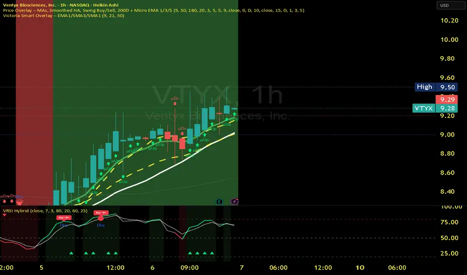
Tristan's Multi-Indicator Reversal StrategyMulti-Indicator Reversal Strategy - Buy Low, Sell High
A comprehensive reversal detection system that combines multiple proven technical indicators to identify high-probability entry points for catching reversals at market extremes.
📊 Strategy Overview
This strategy is designed for traders who want to buy at lows and sell at highs by detecting when stocks are overextended and ready to reverse. It works by requiring multiple technical indicators to align before generating a signal, significantly reducing false entries.
Best Used On:
Timeframe: 1-hour charts (also works on 15min, 30min, 4hour)
Session: NY Trading Session (9:30 AM - 4:00 PM ET)
Assets: Stocks, ETFs, Crypto (particularly volatile tech stocks like ZM, TSLA, AAPL)
Trading Style: Swing trading, Intraday reversals
🔧 Technical Components
The strategy combines FIVE powerful technical indicators:
1. RSI (Relative Strength Index)
2. MACD (Moving Average Convergence Divergence)
3. Williams %R
4. Bollinger Bands
5. Volume Analysis
6. Divergence Detection (Optional)
🎨 Visual Signals
Entry Signals:
🟢 Green Triangle (below candle) = BUY LONG signal
🔴 Red Triangle (above candle) = SELL SHORT signal
Exit Signals:
🟣 Purple Label = Position closed (shows "x2", "x3" if multiple entries)
Additional Indicators:
💎 Aqua Diamond = Bullish divergence detected
💎 Fuchsia Diamond = Bearish divergence detected
🔵 Blue Background = NY Session active
🟡 Yellow Bar Tint = Volume spike detected
⚪ Small Circles = Near-signal conditions (2+ indicators aligned)
Live Counter:
Top corner shows: "Bull: X/4" and "Bear: X/4"
Indicates how many indicators currently align
⚙️ How to Use This Strategy
For Beginners (More Signals):
Set "Min Indicators Aligned" to 2
Turn OFF "Require Divergence"
Turn OFF "Require Volume Spike"
Turn OFF "Require Reversal Candle Pattern"
Keep "Allow Multiple Entries" OFF
This gives you more frequent signals to learn from.
For Advanced Traders (High Probability):
Set "Min Indicators Aligned" to 3 or 4
Turn ON "Require Divergence"
Turn ON "Require Volume Spike"
Turn ON "Require Reversal Candle Pattern"
Adjust stop loss to your risk tolerance
This filters for only the highest-quality setups.
Recommended Settings for 1-Hour Charts:
Min Indicators Aligned: 3
Stop Loss: 2.5%
Take Profit: 5.0%
RSI Length: 14
Williams %R Length: 14
Volume Multiplier: 1.5x
Session: NY only (for stocks)
BUY SIGNAL generated when:
2-4 indicators show oversold/bullish conditions:
RSI < 30 and turning up
MACD crossing bullish or histogram positive
Williams %R < -80 and turning up
Price at/below lower Bollinger Band
Optional confirmations (if enabled):
Bullish divergence detected
Volume spike present
Bullish reversal candle pattern
Session filter: Signals only during NY trading hours
SELL SIGNAL Generated When:
2-4 indicators show overbought/bearish conditions:
RSI > 70 and turning down
MACD crossing bearish or histogram negative
Williams %R > -20 and turning down
Price at/above upper Bollinger Band
Optional confirmations (if enabled):
Bearish divergence detected
Volume spike present
Bearish reversal candle pattern
🛡️ Risk Management Features
Automatic Stop Loss: Protects capital (default 2.5%)
Take Profit Target: Locks in gains (default 5.0%)
Pyramiding Control: Toggle to prevent position stacking
Session Filter: Avoids overnight risk and low-liquidity periods
Position Flipping: Automatically reverses when opposite signal appears
💡 Best Practices
✅ DO:
Wait for candle close before entering (built into strategy)
Use on volatile assets with clear trends
Combine with your own analysis and risk management
Backtest on your specific assets and timeframes
Start with paper trading to learn the signals
Adjust indicator requirements based on market conditions
❌ DON'T:
Use on very low timeframes (<5 min) without adjustment
Ignore the session filter on stocks
Use maximum leverage - these are reversal trades
Trade during major news events or earnings
Expect 100% win rate - focus on risk/reward ratio
📊 Performance Notes
This strategy prioritizes quality over quantity. With default settings, you may see:
2-5 signals per week on 1-hour charts
Higher win rate with stricter settings (3-4 indicators aligned)
Best performance during trending markets with clear reversals
Reduced performance in choppy, sideways markets
Tip: Adjust "Min Indicators Aligned" based on market conditions:
Trending markets: Use 3-4 (fewer but stronger signals)
Range-bound markets: Use 2 (more signals, but watch for false breakouts)

Trend Pullback System```{"variant":"standard","id":"36492","title":"Trend Pullback System Description"}
Trend Pullback System is a price-action trend continuation model that looks to enter on pullbacks, not breakouts. It’s designed to find high-quality long/short entries inside an already established trend, place the stop at meaningful structure, trail that stop as structure evolves, and warn you when the trade thesis is no longer valid.
Developed by: Mohammed Bedaiwi
---------------------------------
HOW IT WORKS
---------------------------------
1. Trend Detection
• The strategy defines overall bias using moving averages.
• Bullish environment (“uptrend”): price above the slower MA, fast MA above slow MA, and the slow MA is sloping up.
• Bearish environment (“downtrend”): price below the slower MA, fast MA below slow MA, and the slow MA is sloping down.
This prevents trading against chop and focuses on continuation moves in the dominant direction.
2. Pullback + Re-entry Logic
• The script waits for price to pull back into structure (support in an uptrend, resistance in a downtrend), and then push back in the direction of the main trend.
• That “push back” is the setup trigger. We don’t chase the first breakout candle — we buy/sell the retest + resume.
3. Structural Levels (“Diamonds”)
• Green diamond (below bar): bullish pivot low formed while the trend is bullish. This marks defended support.
- Use it as a re-entry zone for longs.
- Use it to trail a stop higher when you’re already long.
- Shorts can take profit here because buyers stepped in.
• Red diamond (above bar): bearish pivot high formed while the trend is bearish. This marks defended resistance.
- Use it as a re-entry zone for shorts.
- Use it to trail a stop lower when you’re already short.
- Longs can take profit here because sellers stepped in.
4. Entry Signals
• BUY arrow (green triangle up under the candle, text like “BUY” / “BUY Zone”):
- LongSetup is true.
- Trend is bullish or turning bullish.
- Price just bounced off recent defended support (green diamond) and reclaimed short-term momentum.
Meaning: enter long here or cover/exit shorts.
• SELL arrow (red triangle down above the candle):
- ShortSetup is true.
- Trend is bearish or turning bearish.
- Price just rolled down from defended resistance (red diamond) and lost short-term momentum.
Meaning: enter short here or take profit on longs.
These are the primary trade entries. They are meant to be actionable.
5. Weak Setups (“W” in yellow)
• Yellow triangle with “W”:
- A possible long/short idea is trying to form, BUT the higher-timeframe confirmation is not fully there yet.
- Think of it as early pressure / early caution, not a full signal.
• You usually watch these areas rather than jumping in immediately.
6. Exit Warning (orange “EXIT” label above a bar)
• The strategy will raise an EXIT marker when you’re in a trade and the *opposite* side just produced a confirmed setup.
- You’re short and a valid longSetup appears → EXIT.
- You’re long and a valid shortSetup appears → EXIT.
• This is basically: “Close or reduce — the other side just took control.”
• It’s not just a trailing stop hit; it’s a regime flip warning.
7. Stop, Target, and Trailing
• On every new setup, the script records:
- Initial stop: recent swing beyond the defended level (below support for longs, above resistance for shorts).
- Initial target: recent opposing swing.
• While you’re in position, if new confirming diamonds print in your favor, the stop can trail toward the new defended level.
• This creates structure-based risk management (not just fixed % or ATR).
8. Reference Levels
• The strategy also plots prior higher-timeframe closes (last week’s close, last month’s close, last year’s close). These can behave as magnets or stall points.
• They’re helpful for take-profit timing and for reading “are we trading above or below last month’s close?”
9. Momentum Panel (hidden by default)
• Internally, the script calculates an SMI-style momentum oscillator with overbought/oversold zones.
• This is optional visual confirmation and does not drive the core entry/exit logic.
---------------------------------
WHAT A TRADE LOOKS LIKE IN REAL PRICE ACTION
---------------------------------
Early warning
• Yellow W + red diamonds + red down arrows = “This is getting weak. Short setups are here.”
• You may also see something like “My Short Entry Id.” That’s where the short side actually engages.
Bearish follow-through, then exhaustion
• Price bleeds down.
• Then the orange EXIT appears.
→ Translation: “If you’re still short, close it. Buyers are stepping in hard. Risk of reversal is now high.”
Regime flip
• Right after EXIT, multiple green BUY arrows fire together (“BUY”, “BUYZone”).
• That’s the true long trigger.
→ This is where you either enter long or flip from short to long.
Expansion leg
• After that flip, price rips up for multiple candles / days / weeks.
• While it runs:
- Green diamonds appear under pullbacks → “dip buy zones / trail stop up here.”
- More BUY arrows show on minor pullbacks → continuation long / scale adds.
Distribution / topping
• Later, you start seeing new yellow W triangles again near local highs. That’s your “careful, this might be topping” warning.
• You finally get a hard red candle, and green diamonds stop stacking.
→ That’s where you tighten risk, scale out, or assume the move is mature.
In plain terms, the model is doing the following for you:
• It puts you short during weakness.
• It tells you when to get OUT of the short.
• It flips you long right as control changes.
• It gives you a structure-based trail the whole way up.
• It warns you again when momentum at the top starts cracking.
That is exactly how the logic was designed.
---------------------------------
QUICK INTERPRETATION CHEAT SHEET
---------------------------------
🔻 Red triangle + “Short Entry” near a red diamond
→ Short entry zone (or take profit on a long).
🟥 Red diamond above bar
→ Sellers defended here. Treat it as resistance. Good place to trail short stops just above that level. Avoid chasing longs straight into it.
🟨 Yellow W
→ Attention only. Early pressure / possible turn. Not fully confirmed.
🟧 EXIT (orange label)
→ The opposite side just printed a real setup. Close the old idea (cover shorts if you’re short, exit longs if you’re long). Thesis invalid.
🟩 Burst of green BUY triangles after EXIT
→ Long entry. Also a “cover shorts now” alert. This is the core money entry in bullish reversals.
💎 Green diamond below bar
→ Bulls defended that level. Good for trailing your long stop up, and good “buy the dip in trend” locations.
📈 Blue / teal MAs stacked and rising
→ Confirmed bullish structure. You’re in trend continuation mode, so dips are opportunities, not automatic exits.
---------------------------------
COLOR / SHAPE KEY
---------------------------------
• Green triangle up (“BUY”, “BUY Zone”):
Long entry / cover shorts / continuation long trigger.
• Red triangle down:
Short entry / take profit on longs / continuation short trigger.
• Orange “EXIT” label:
Opposite side just fired a real setup. The previous trade thesis is now invalid.
• Green diamond below price:
Bullish defended support in an uptrend. Use for dip buys, trailing stops on longs, and objective cover zones for shorts.
• Red diamond above price:
Bearish defended resistance in a downtrend. Use for re-entry shorts, trailing stops on shorts, and objective scale-out zones for longs.
• Yellow “W”:
Weak / early potential setup. Watch it, don’t blindly trust it.
• Moving average bands (fast MA, slow MA, Hull MA):
When stacked and rising, bullish control. When stacked and falling, bearish control.
---------------------------------
INTENT
---------------------------------
This system is built to:
• Trade with momentum, not against it.
• Enter on pullbacks into proven structure, not chase stretched breakouts.
• Automate stop/target logic around actual defended swing levels.
• Warn you when the other side takes over so you don’t give back gains.
Typical usage:
1. In an uptrend, wait for price to pull back, print a green diamond (support proved), then take the first BUY arrow that fires.
2. In a downtrend, wait for a bounce into resistance, print a red diamond (sellers proved), then take the first SELL arrow that fires.
3. Respect EXIT when it appears — that’s the model saying “this trade is done.”
---------------------------------
DISCLAIMER
---------------------------------
This script is for educational and research purposes only. It is not financial advice, investment advice, or a recommendation to buy or sell any security, cryptoasset, or derivative. Markets carry risk. Past performance does not guarantee future results. You are fully responsible for your own decisions, position sizing, risk management, and compliance with all applicable laws and regulations.

[Kpt-Ahab] Assistant: Risk & DCA PlannerScript Description – Assistant: Risk & DCA Planner
The Risk & DCA Planner is a technical assistant for position and risk management.
It automatically calculates, based on volatility (ATR%), swing structure, and your settings:
Stop-Loss (SL) and corresponding Take-Profit targets (TPs) in R-multiples
DCA (Dollar-Cost-Averaging) levels — both price and amount
A market suitability check (based on volatility & volume)
Plus a clear table and summary label displayed on the chart
The script helps you plan risk, scaling, and profit targets consistently and quantitatively.
Core Logic
Risk Profile
Three modes: Low, Normal, High.
These define how reactive the script behaves internally:
Low → conservative, longer lookbacks, tighter analysis
Normal → balanced
High → aggressive, faster reaction, wider stops
Stop-Loss (SL)
Automatically calculated from ATR% and recent swing structure, limited by minimum and maximum thresholds.
The SL percentage defines the R-unit, which all TPs and DCA levels are based on.
Take-Profits (TPs)
Up to six targets, each a multiple of the defined risk (e.g., 1R, 2R, 3R).
Prices are automatically adjusted depending on long or short direction.
DCA Strategy
Optional. Adds scaling levels evenly between Entry and SL or in multiples of the ATR.
Each DCA allocation grows geometrically until the maximum position size is reached.
Suitability Check
Evaluates whether the market is within an appropriate ATR% range and has sufficient volume.
The table displays “OK” or “Caution” depending on volatility and historical consistency.
Visualization
Lines for SL, TPs, and DCA levels
A table with all parameters, prices, and risk data
A chart label summarizing key info (profile, direction, SL%, TPs, DCA, etc.)

Advanced Multi-Timeframe Trend & Signal System═══════════════════════════════════════════════════════════════
ADVANCED MULTI-TIMEFRAME TREND & SIGNAL SYSTEM v1.0
═══════════════════════════════════════════════════════════════
Created by: Zakaria Safri
License: Mozilla Public License 2.0
A comprehensive technical analysis tool designed for traders seeking
multi-dimensional market insights. This indicator combines proven
technical analysis methods with modern visualization techniques.
═══════════════════════════════════════════════════════════════
KEY FEATURES
═══════════════════════════════════════════════════════════════
✓ SUPERTREND SIGNAL GENERATION
- Customizable sensitivity settings
- Clear long/short entry signals
- Automatic trend direction detection
- ATR-based dynamic calculations
✓ MULTI-TIMEFRAME DASHBOARD
- Real-time trend analysis across 6 timeframes
- Synchronized trend confirmation
- Customizable table position and size
- Current: 1M, 5M, 15M, 1H, 1D coverage
✓ QQE REVERSAL DETECTION
- Quantitative Qualitative Estimation algorithm
- Early reversal signal identification
- Adjustable RSI and smoothing parameters
- Confirmation-based plotting
✓ DYNAMIC SUPPORT & RESISTANCE
- Pivot-based level calculation
- Quick and standard pivot detection
- Color-coded zones (8 levels)
- Automatic level updates
✓ MOMENTUM BREAKOUT SIGNALS
- Ichimoku-inspired calculations
- Bullish and bearish breakout detection
- Visual zone highlighting
- Trend confirmation filters
✓ RISK MANAGEMENT SYSTEM
- ATR-based stop loss calculation
- Multiple take profit targets (TP1, TP2, TP3)
- Customizable risk-to-reward ratios
- Dynamic price level tracking
- Hit detection markers
✓ VOLATILITY BANDS
- Keltner Channel implementation
- Multiple band layers (3 levels)
- EMA-based calculations
- Adaptive to market conditions
✓ TREND CLOUD VISUALIZATION
- Dual moving average cloud
- Clear trend direction indication
- Customizable color scheme
- Trend bar coloring
═══════════════════════════════════════════════════════════════
HOW TO USE
═══════════════════════════════════════════════════════════════
SETUP:
1. Add indicator to your chart
2. Configure sensitivity in Core Signals section
3. Enable desired features (signals, reversals, breakouts)
4. Set up risk management levels if trading
5. Position MTF dashboard to preference
SIGNAL INTERPRETATION:
• LONG Signal: Price crosses above Supertrend
• SHORT Signal: Price crosses below Supertrend
• REV (Reversal): QQE indicates potential trend change
• Diamond Breakouts: Momentum shift confirmation
• T1/T2/T3: Take profit level hits
MULTI-TIMEFRAME ANALYSIS:
• Green (BULL): Higher timeframe supports uptrend
• Red (BEAR): Higher timeframe supports downtrend
• Use for trend alignment and confirmation
• Best results when multiple timeframes align
RISK MANAGEMENT:
• Enable Stop Loss for automatic SL calculation
• Activate TP levels based on trading style
• Adjust Risk-to-Reward ratio (1:1 to 1:10)
• Monitor hit detection circles for exits
═══════════════════════════════════════════════════════════════
TECHNICAL SPECIFICATIONS
═══════════════════════════════════════════════════════════════
CALCULATIONS:
• Supertrend: ATR-based with customizable multiplier
• QQE: Modified RSI with Wilders smoothing
• Keltner Channels: EMA basis with ATR bands
• Pivots: Standard left/right bar methodology
• Support/Resistance: Multi-level pivot analysis
PARAMETERS:
• Supertrend Sensitivity: 0.5 to 10.0 (default: 2.0)
• RSI Period: 5 to 50 (default: 14)
• QQE Multiplier: 1.0 to 10.0 (default: 4.238)
• Risk-to-Reward: 1 to 10 (default: 4)
TIMEFRAMES:
Compatible with all timeframes. MTF dashboard displays:
• 1 Minute (1M)
• 5 Minutes (5M)
• 15 Minutes (15M)
• 1 Hour (1H)
• 1 Day (1D)
• Current chart timeframe
═══════════════════════════════════════════════════════════════
CUSTOMIZATION OPTIONS
═══════════════════════════════════════════════════════════════
VISUAL:
• Professional color scheme (Cyan/Orange)
• Adjustable table position (9 positions)
• Table size options (tiny/small/normal/large)
• Transparent zone highlighting
• Clean, modern label design
TOGGLES:
• Enable/disable any feature independently
• Show/hide signals, reversals, breakouts
• Toggle S/R levels and zones
• Control trend cloud and bands
• Master trend line optional
ALERTS:
The indicator provides visual signals that can be used with
TradingView's alert system by setting alerts on the indicator.
═══════════════════════════════════════════════════════════════
BEST PRACTICES
═══════════════════════════════════════════════════════════════
✓ Combine signals for higher probability setups
✓ Use MTF dashboard for trend confirmation
✓ Respect S/R levels for entry/exit planning
✓ Monitor QQE reversals at key price levels
✓ Adjust sensitivity based on asset volatility
✓ Test on demo/paper trading first
✓ Use proper risk management always
═══════════════════════════════════════════════════════════════
IMPORTANT DISCLAIMER
═══════════════════════════════════════════════════════════════
This indicator is a technical analysis tool and does NOT:
• Guarantee profitable trades
• Provide financial advice
• Predict future price movements with certainty
• Replace proper risk management
• Substitute for personal due diligence
Past performance does not indicate future results. All trading
involves risk. Users should:
- Understand the indicator's logic
- Test thoroughly before live trading
- Use appropriate position sizing
- Never risk more than they can afford to lose
- Consult financial advisors if needed
═══════════════════════════════════════════════════════════════
CODING STANDARDS
═══════════════════════════════════════════════════════════════
This indicator follows PineCoders Coding Conventions:
✓ Proper variable naming (prefixes: i_, f_, c_)
✓ Clear function documentation
✓ Organized code structure
✓ Type declarations
✓ Efficient calculations
✓ No repainting (confirmed signals)
✓ Proper use of request.security
═══════════════════════════════════════════════════════════════
SUPPORT & UPDATES
═══════════════════════════════════════════════════════════════
Version: 1.0
Author: Zakaria Safri
License: MPL 2.0
Last Updated: 2024
For questions, feedback, or suggestions, please comment below.
═══════════════════════════════════════════════════════════════
#trading #signals #supertrend #multiTimeframe #QQE #reversals
#supportResistance #riskManagement #trendAnalysis #momentum
